more e’s [and R’s]
 Alex Thiéry suggested debiasing the biased estimate of e by Rhee and Glynn truncated series method, so I tried the method to see how much of an improvement (if any!) this would bring. I first attempted to naïvely implement the raw formula of Rhee and Glynn

with a (large) Poisson distribution on the stopping rule N, but this took ages. I then realised that the index n did not have to be absolute, i.e. to start at n=1 and proceed snailwise one integer at a time: the formula remains equally valid after a change of time, i.e. n=can start at an arbitrary value and proceeds by steps of arbitrary size, which obviously speeds things up!
n=1e6
step=1e2
lamb=1e2
rheest=function(use=runif(n)){
rest=NULL
pond=rpois(n,lamb)+1
imax=min(which((1:n)>n-pond))
i=1
while (i<=imax){
 m=pond[i]
 teles=past=0
 for (j in 1:m){
  space=mean(j*diff(sort(use[i:(i+step*j)]))>.01)
  if (space>0){ space=1/space}
     else{ space=3}
  teles=teles+(space-past)/(1-ppois(j-1,lamb))
  past=space
  }
 rest=c(rest,teles)
 i=i+step*m+1}
return(rest)}
For instance, the running time of the above code with n=10⁶ uniforms in use is
> system.time(mean(rheest(runif(n))))
utilisateur     système      écoulé
      6.035       0.000       6.031
If I leave aside the issue of calibrating the above in terms of the Poisson parameter λ and of the step size [more below!], how does this compare with Forsythe’s method? Very (very) well if following last week pedestrian implementation:
> system.time(mean(forsythe(runif(n))))
utilisateur     système      écoulé
    146.115       0.000     146.044
But then I quickly (not!) realised that proceeding sequentially through the sequence of uniform simulations was not necessary to produce independent realisations of Forsythe’s estimate: this R code takes batches of uniforms that are far enough to see a sign change in the differences and takes the length of the first decreasing sequence for each batch. While this certainly is suboptimal in exploiting the n Uniform variates, it avoids scrawling through the sequence one value at a time and is clearly way faster:
fastythe=function(use=runif(n)){
  band=max(diff((1:(n-1))[diff(use)>0]))+1
  bends=apply(apply((apply(matrix(use[1:((n%/%band)*band)],
    nrow=band),2,diff)<0),2,cumprod),2,sum)}

> system.time(mean(fastythe()))
utilisateur     système      écoulé
      0.904       0.000       0.903
while producing much more accurate estimates than the debiased version if not the original one, as shown by the boxplot at the top (where RG stands for Rhee and Glynn, F for Forsythe and W for Wuber who proposed the original [biased] Monte Carlo estimate of e⁻¹)! Just to make things clear if necessary, all comparisons are run with the same batch of 10⁶ uniform simulations for each mean value entering the boxplots.
One thing that bothers me about the debiased solution is that it is highly sensitive to calibration. For instance, when switching λ and the step size between 10 and 100, I got the following variation over 100 replicates:
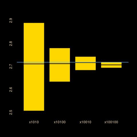 where the last box corresponds to the RG box on the first graph. This is most annoying in that using the whole sequence of uniforms at once and the resulting (biased) estimator leads to the most precise and fastest estimator of the whole series (W label in the first graph)!
> system.time(1/mean((n-1)*diff(sort(use))>1))
utilisateur     système      écoulé
      0.165       0.000       0.163

February 22, 2016 at 5:03 am
[…] article was first published on R – Xi’an’s Og , and kindly contributed […]