the demise of the Bayes factor

With Kaniav Kamary, Kerrie Mengersen, and Judith Rousseau, we have just arXived (and submitted) a paper entitled “Testing hypotheses via a mixture model”. (We actually presented some earlier version of this work in Cancũn, Vienna, and Gainesville, so you may have heard of it already.) The notion we advocate in this paper is to replace the posterior probability of a model or an hypothesis with the posterior distribution of the weights of a mixture of the models under comparison. That is, given two models under comparison,

we propose to estimate the (artificial) mixture model

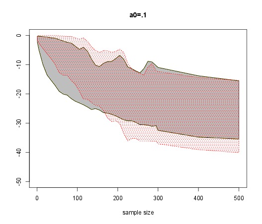
and in particular derive the posterior distribution of α. One may object that the mixture model is neither of the two models under comparison but this is the case at the boundary, i.e., when α=0,1. Thus, if we use prior distributions on α that favour the neighbourhoods of 0 and 1, we should be able to see the posterior concentrate near 0 or 1, depending on which model is true. And indeed this is the case: for any given Beta prior on α, we observe a higher and higher concentration at the right boundary as the sample size increases. And establish a convergence result to this effect. Furthermore, the mixture approach offers numerous advantages, among which [verbatim from the paper]:

• relying on a Bayesian estimator of the weight α rather than on the posterior probability of the corresponding model does remove the need of overwhelmingly artificial prior probabilities on model indices;
•  the interpretation of this estimator is at least as natural as handling the posterior probability, while avoiding the caricaturesque zero-one loss setting. The quantity α and its posterior distribution provide a measure of proximity to both models for the data at hand, while being also interpretable as a propensity of the data to stand with (or to stem from) one of the two models. This representation further allows for alternative perspectives on testing and model choices, through the notions of predictive tools  cross-validation, and information indices like WAIC;
• the highly problematic computation of the marginal likelihoods is bypassed, standard algorithms being available for Bayesian mixture estimation;
• the extension to a finite collection of models to be compared is straightforward, as this simply involves a larger number of components. This approach further allows to consider all models at once rather than engaging in pairwise costly comparisons and thus to eliminate the least likely models by simulation, those being not explored by the corresponding algorithm;
• the (simultaneously conceptual and computational) difficulty of “label switching” that plagues both Bayesian estimation and Bayesian computation for most mixture models completely vanishes in this particular context, since components are no longer exchangeable. In particular, we compute neither a Bayes factor nor a posterior probability related with the substitute mixture model and we hence avoid the difficulty of recovering the modes of the posterior distribution. Our perspective is solely centred on estimating the parameters of a mixture model where both components are always identifiable;
• the posterior distribution of α evaluates more thoroughly the strength of the support for a given model than the single figure outcome of a Bayes factor or of a posterior probability. The variability of the posterior distribution on α allows for a more thorough assessment of the strength of the support of one model against the other;
• an additional feature missing from traditional Bayesian answers is that a mixture model also acknowledges the possibility that, for a finite dataset, both models or none could be acceptable.
• while standard (proper and informative) prior modelling can be painlessly reproduced in this novel setting, non-informative (improper) priors now are manageable therein, provided both models under comparison are first reparametrised towards common-meaning and shared parameters, as for instance with location and scale parameters. In the special case when all parameters can be made common to both models [While this may sound like an extremely restrictive requirement in a traditional mixture model, let us stress here that the presence of common parameters becomes quite natural within a testing setting. To wit, when comparing two different models for the same data, moments are defined in terms of the observed data and hence should be the same for both models. Reparametrising the models in terms of those common meaning moments does lead to a mixture model with some and maybe all common parameters. We thus advise the use of a common parametrisation, whenever possible.] the mixture model reads as

  

  For instance, if θ is a location parameter, a flat prior can be used with no foundational difficulty, in opposition to the testing case;

• continuing from the previous argument, using the same parameters or some identical parameters on both components is an essential feature of this reformulation of Bayesian testing, as it highlights the fact that the opposition between the two components of the mixture is not an issue of enjoying different parameters, but quite the opposite. As further stressed below, this or even those common parameter(s) is (are) nuisance parameters that need be integrated out (as they also are in the traditional Bayesian approach through the computation of the marginal likelihoods);
• the choice of the prior model probabilities is rarely discussed in a classical Bayesian approach, even though those probabilities linearly impact the posterior probabilities and can be argued to promote the alternative of using the Bayes factor instead. In the mixture estimation setting, prior modelling only involves selecting a prior on α, for instance a Beta B(a,a) distribution, with a wide range of acceptable values for the hyperparameter a. While the value of a impacts the posterior distribution of α, it can be argued that (a) it nonetheless leads to an accumulation of the mass near 1 or 0, i.e., to favour the most favourable or the true model over the other one, and (b) a sensitivity analysis on the impact of a is straightforward to carry on;
• in most settings, this approach can furthermore be easily calibrated by a parametric bootstrap experiment providing a posterior distribution of α under each of the models under comparison. The prior predictive error can therefore be directly estimated and can drive the choice of the hyperparameter a, if need be.