an ABC experiment

 

In a cross-validated forum exchange, I used the code below to illustrate the working of an ABC algorithm:

#normal data with 100 observations
n=100
x=rnorm(n)
#observed summaries
sumx=c(median(x),mad(x))

#normal x gamma prior
priori=function(N){
 return(cbind(rnorm(N,sd=10),
  1/sqrt(rgamma(N,shape=2,scale=5))))
}

ABC=function(N,alpha=.05){

  prior=priori(N) #reference table

  #pseudo-data
  summ=matrix(0,N,2)
  for (i in 1:N){
   xi=rnorm(n)*prior[i,2]+prior[i,1]
   summ[i,]=c(median(xi),mad(xi)) #summaries
   }

  #normalisation factor for the distance
  mads=c(mad(summ[,1]),mad(summ[,2]))
  #distance
  dist=(abs(sumx[1]-summ[,1])/mads[1])+
   (abs(sumx[2]-summ[,2])/mads[2])
  #selection
  posterior=prior[dist<quantile(dist,alpha),]}

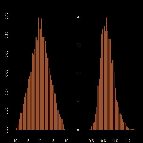
Hence I used the median and the mad as my summary statistics. And the outcome is rather surprising, for two reasons: the first one is that the posterior on the mean μ is much wider than when using the mean and the variance as summary statistics. This is not completely surprising in that the latter are sufficient, while the former are not. Still, the (-10,10) range on the mean is way larger… The second reason for surprise is that the true posterior distribution cannot be derived since the joint density of med and mad is unavailable.

After thinking about this for a while, I went back to my workbench to check the difference with using mean and variance. To my greater surprise, I found hardly any difference! Using the almost exact ABC with 10⁶ simulations and a 5% subsampling rate returns exactly the same outcome. (The first row above is for the sufficient statistics (mean,standard deviation) while the second row is for the (median,mad) pair.) Playing with the distance does not help. The genuine posterior output is quite different, as exposed on the last row of the above, using a basic Gibbs sampler since the posterior is not truly conjugate.