a [counter]example of minimaxity

A chance question on X validated made me reconsider about the minimaxity over the weekend. Consider a Geometric G(p) variate X. What is the minimax estimator of p under squared error loss ? I thought it could be obtained via (Beta) conjugate priors, but following Dyubin (1978) the minimax estimator corresponds to a prior with point masses at ¼ and 1, resulting in a constant estimator equal to ¾ everywhere, except when X=0 where it is equal to 1. The actual question used a penalised qaudratic loss, dividing the squared error by p(1-p), which penalizes very strongly errors at p=0,1, and hence suggested an estimator equal to 1 when X=0 and to 0 otherwise. This proves to be the (unique) minimax estimator. With constant risk equal to 1. This reminded me of this fantastic 1984 paper by Georges Casella and Bill Strawderman on the estimation of the normal bounded mean, where the least favourable prior is supported by two atoms if the bound is small enough. Figure 1 in the Negative Binomial extension by Morozov and Syrova (2022) exploits the same principle. (Nothing Orwellian there!) If nothing else, a nice illustration for my Bayesian decision theory course!

Xing glass bridges [or not]

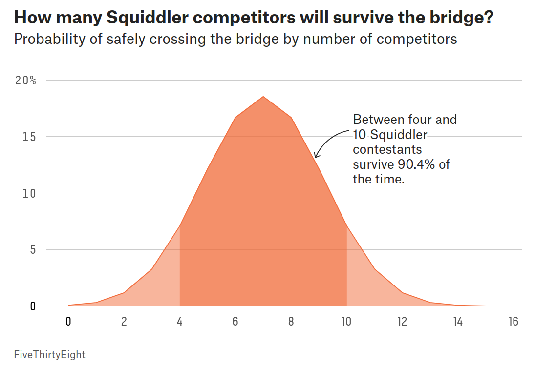
A riddle from the Riddler surfing on Squid Games. Evaluating the number of survivors (out of 16 players) able to X the glass bridge, when said bridge is made of 18 consecutive steps, each involving a choice between a tempered and a non-tempered glass square. Stepping on a non-tempered square means death, while all following players are aware of the paths of the earlier ones. Each player thus moves at least one step further than the previous and unlucky player. The total number of steps used by the players is therefore a Negative Binomial Neg(16,½) variate truncated at 19 (if counting attempts rather than failures), with the probability of reaching 19 being .999. When counting the number of survivors, a direct simulation gives an estimate very close to 7:

   mean(apply(apply(matrix(rgeom(16*1e6,.5)+1,nc=16),1,cumsum)>18,2,sum))

but the expectation is not exactly 7! Indeed, this value is a sum of probabilities that the cumulated sums of Geometric variates are larger than 18, which has no closed form as far as I can see

   sum(1-pnbinom(size=1:16,q=17:2,prob=.5)

but whose value is 7.000076. In the Korean TV series, there are only three survivors, which would have had a .048 probability of occurring. (Not accounting for the fact that one player was temporarily able to figure out which square was right and that two players fell through at the same time.)

Looking later at on-line discussions, I found that the question was quite popular, with a whole spectrum of answers… Including a wrong Binomial B(18, ½) modelling that does not account for the fact that all 16 (incredibly unlucky) players could have died before the last steps.

And reading the solution on The Riddler a week later, I was sorry to see this representation of the distribution of survivors, as if it was a continuous distribution!

maximum likelihood on negative binomial

Estimating both parameters of a negative binomial distribution NB(N,p) by maximum likelihood sounds like an obvious exercise. But it is not because some samples lead to degenerate solutions, namely p=0 and N=∞… This occurs when the mean of the sample is larger than its empirical variance, s²>x̄, not an impossible instance: I discovered this when reading a Cross Validated question asking about the action to take in such a case. A first remark of interest is that this only happens when the negative binomial distribution is defined in terms of failures (since else the number of successes is bounded). A major difference I never realised till now, for estimating N is not a straightforward exercise. A second remark is that a negative binomial NB(N,p) is a Poisson compound of an LSD variate with parameter p, the Poisson being with parameter η=-N log(1-p). And the LSD being a power distribution p^k/k rather than a psychedelic drug. Since this is not an easy framework, Adamidis (1999) introduces an extra auxiliary variable that is a truncated exponential on (0,1) with parameter -log(1-p). A very neat trick that removes the nasty normalising constant on the LSD variate.

“Convergence was achieved in all cases, even when the starting values were poor and this emphasizes the numerical stability of the EM algorithm.” K. Adamidis

Adamidis then constructs an EM algorithm on the completed set of auxiliary variables with a closed form update on both parameters. Unfortunately, the algorithm only works when s²>x̄. Otherwise, it gets stuck at the boundary p=0 and N=∞. I was hoping for a replica of the mixture case where local maxima are more interesting than the degenerate global maximum… (Of course, there is always the alternative of using a Bayesian noninformative approach.)

Rasmus’ socks fit perfectly!

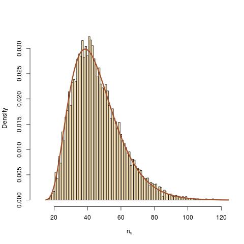Following the previous post on Rasmus’ socks, I took the opportunity of a survey on ABC I am currently completing to compare the outcome of his R code with my analytical derivation. After one quick correction [by Rasmus] of a wrong representation of the Negative Binomial mean-variance parametrisation [by me], I achieved this nice fit…

the alive particle filter

As mentioned earlier on the ‘Og, this is a paper written by Ajay Jasra, Anthony Lee, Christopher Yau, and Xiaole Zhang that I missed when it got arXived (as I was also missing my thumb at the time…) The setting is a particle filtering one with a growing product of spaces and constraints on the moves between spaces. The motivating example is one of an ABC algorithm for an HMM where at each time, the simulated (pseudo-)observation is forced to remain within a given distance of the true observation. The (one?) problem with this implementation is that the particle filter may well die out by making only proposals that stand out of the above ball. Based on an idea of François Le Gland and Nadia Oudjane, the authors define the alive filter by imposing a fixed number of moves onto the subset, running a negative binomial number of proposals. By removing the very last accepted particle, they show that the negative binomial experiment allows for an unbiased estimator of the normalising constant(s). Most of the paper is dedicated to the theoretical study of this scheme, with results summarised as (p.2)

1. Time uniform L_p bounds for the particle filter estimates
2. A central limit theorem (CLT) for suitably normalized and centered particle filter estimates
3. An unbiased property of the particle filter estimates
4. The relative variance of the particle filter estimates, assuming N = O(n), is shown to grow linearly in n.

The assumptions necessary to reach those impressive properties are fairly heavy (or “exceptionally strong” in the words of the authors, p.5): the original and constrained transition kernels are both uniformly ergodic, with equivalent coverage of the constrained subsets for all possible values of the particle at the previous step. I also find the proposed implementation of the ABC filtering inadequate for approximating the posterior on the parameters of the (HMM) model. Expecting every realisation of the simulated times series to be close to the corresponding observed value is too hard a constraint. The above results are scaled in terms of the number N of accepted particles but it may well be that the number of generated particles and hence the overall computing time is much larger. In the examples completing the paper, the comparison is run with an earlier ABC sampler based on the very same stepwise proximity to the observed series so the impact of this choice is difficult to assess and, furthermore, the choice of the tolerances ε is difficult to calibrate: is 3, 6, or 12 a small or large value for ε? A last question that I heard from several sources during talks on that topic is why an ABC approach would be required in HMM settings where SMC applies. Given that the ABC reproduces a simulation on the pair latent variables x parameters, there does not seem to be a gain there…