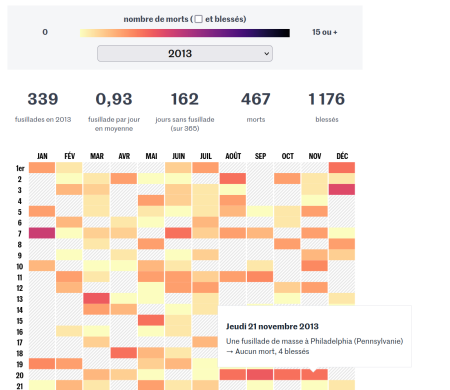
max spacing between mass shootings [data graphics]

simulating the maximum of Rayleigh variates

An X validated question on an efficient way to simulate the largest order statistics of a Rayleigh (large) sample. Named after the 1904 Nobel recipient, John Strutt. This is not a commonly used distribution in statistics, since it coincides with the χ₂ distribution. Anyway, thanks to its compact, closed form cdf, the largest order statistics can be directly simulated, at a constant cost in the sample size, as

or equivalently as

since the smallest order statistic from a Uniform sample, U₍₁₎, is distributed from a  Be(1,N) distribution.

where is .5?

A Riddler’s riddle on breaking the unit interval into 4 random bits (by which I understand picking 3 Uniform realisations and ordering them) and finding the length of the bit containing ½ (sparing you the chore of converting inches and feet into decimals). The result can be found by direct integration since the ordered Uniform variates are Beta’s, and so are their consecutive differences, leading to an average length of 15/32. Or by raw R simulation:

simz=t(apply(matrix(runif(3*1e5),ncol=3),1,sort))
mean((simz[,1]>.5)*simz[,1]+
  (simz[,1]<.5)*(simz[,2]>.5)*(simz[,2]-simz[,1])+
  (simz[,2]<.5)*(simz[,3]>.5)*(simz[,3]-simz[,2])+
  (simz[,3]<.5)*(1-simz[,3]))

Which can be reproduced for other values than ½, showing that ½ is the value leading to the largest expected length. I wonder if there is a faster way to reach this nice 15/32.

easy Riddler

The riddle of the week is rather standard probability calculus

If N points are generated at random places on the perimeter of a circle, what is the probability that you can pick a diameter such that all of those points are on only one side of the newly halved circle?

Since it is equivalent to finding the range of N Uniform variates less than ½. And since the range of N Uniform variates is distributed as a Be(N-1,2) random variate. The resulting probability, which happens to be exactly , is decreasing exponentially, as shown below…

Example 7.3: what a mess!

A rather obscure question on Metropolis-Hastings algorithms on X Validated ended up being about our first illustration in Introducing Monte Carlo methods with R. And exposing some inconsistencies in the following example… Example 7.2 is based on a [toy] joint Beta x Binomial target, which leads to a basic Gibbs sampler. We thought this was straightforward, but it may confuse readers who think of using Gibbs sampling for posterior simulation as, in this case, there is neither observation nor posterior, but simply a (joint) target in (x,θ).

And then it indeed came out that we had incorrectly written Example 7.3 on the [toy] Normal posterior, using at times a Normal mean prior with a [prior] variance scaled by the sampling variance and at times a Normal mean prior with a [prior] variance unscaled by the sampling variance. I am rather amazed that this did not show up earlier. Although there were already typos listed about that example.