the Flatland paradox [#2]

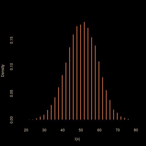
Another trip in the métro today (to work with Pierre Jacob and Lawrence Murray in a Paris Anticafé!, as the University was closed) led me to infer—warning!, this is not the exact distribution!—the distribution of x, namely

since a path x of length l(x) will corresponds to N draws if N-l(x) is an even integer 2p and p undistinguishable annihilations in 4 possible directions have to be distributed over l(x)+1 possible locations, with Feller’s number of distinguishable distributions as a result. With a prior π(N)=1/N on N, hence on p, the posterior on p is given by

Now, given N and  x, the probability of no annihilation on the last round is 1 when l(x)=N and in general

which can be integrated against the posterior. The numerical expectation is represented for a range of values of l(x) in the above graph. Interestingly, the posterior probability is constant for l(x) large  and equal to 0.8125 under a flat prior over N.

Getting back to Pierre Druilhet’s approach, he sets a flat prior on the length of the path θ and from there derives that the probability of annihilation is about 3/4. However, “the uniform prior on the paths of lengths lower or equal to M” used for this derivation which gives a probability of length l proportional to 3^l is quite different from the distribution of l(θ) given a number of draws N. Which as shown above looks much more like a Binomial B(N,1/2).

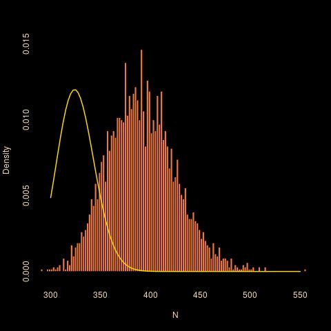However, being not quite certain about the reasoning involving Fieller’s trick, I ran an ABC experiment under a flat prior restricted to (l(x),4l(x)) and got the above, where the histogram is for a posterior sample associated with l(x)=195 and the gold curve is the potential posterior. Since ABC is exact in this case (i.e., I only picked N’s for which l(x)=195), ABC is not to blame for the discrepancy! I asked about the distribution on Stack Exchange maths forum (and a few colleagues here as well) but got no reply so far… Here is the R code that goes with the ABC implementation:

#observation:
elo=195
#ABC version
T=1e6
el=rep(NA,T)
N=sample(elo:(4*elo),T,rep=TRUE)
for (t in 1:T){
#generate a path
  paz=sample(c(-(1:2),1:2),N[t],rep=TRUE)
#eliminate U-turns
  uturn=paz[-N[t]]==-paz[-1]
  while (sum(uturn>0)){
    uturn[-1]=uturn[-1]*(1-
              uturn[-(length(paz)-1)])
    uturn=c((1:(length(paz)-1))[uturn==1],
            (2:length(paz))[uturn==1])
    paz=paz[-uturn]
    uturn=paz[-length(paz)]==-paz[-1]
    }
  el[t]=length(paz)}
#subsample to get exact posterior
poster=N[abs(el-elo)==0]

the Flatland paradox

Pierre Druilhet arXived a note a few days ago about the Flatland paradox (due to Stone, 1976) and his arguments against the flat prior. The paradox in this highly artificial setting is as follows:  Consider a sequence θ of N independent draws from {a,b,1/a,1/b} such that

1. N and θ are unknown;
2. a draw followed by its inverse and this inverse are removed from θ;
3. the successor x of θ is observed, meaning an extra draw is made and the above rule applied.

Then the frequentist probability that x is longer than θ given θ is at least 3/4—at least because θ could be zero—while the posterior probability that x is longer than θ given x is 1/4 under the flat prior over θ. Paradox that 3/4 and 1/4 clash. Not so much of a paradox because there is no joint probability distribution over (x,θ).

The paradox was actually discussed at length in Larry Wasserman’s now defunct Normal Variate. From which I borrowed Larry’s graphical representation of the four possible values of θ given the (green) endpoint of x. Larry uses the Flatland paradox hammer to fix another nail on the coffin he contemplates for improper priors. And all things Bayes. Pierre (like others before him) argues against the flat prior on θ and shows that a flat prior on the length of θ leads to recover 3/4 as the posterior probability that x is longer than θ.

As I was reading the paper in the métro yesterday morning, I became less and less satisfied with the whole analysis of the problem in that I could not perceive θ as a parameter of the model. While this may sound a pedantic distinction, θ is a latent variable (or a random effect) associated with x in a model where the only unknown parameter is N, the total number of draws used to produce θ and x. The distributions of both θ and x are entirely determined by N. (In that sense, the flatland paradox can be seen as a marginalisation paradox in that an improper prior on N cannot be interpreted as projecting a prior on θ.) Given N, the distribution of x of length l(x) is then 1/4^N times the number of ways of picking (N-l(x)) annihilation steps among N. Using a prior on N like 1/N , which is improper, then leads to favour the shortest path as well. (After discussing the issue with Pierre Druilhet, I realised he had a similar perspective on the issue. Except that he puts a flat prior on the length l(x).) Looking a wee bit further for references, I also found that Bruce Hill had adopted the same perspective of a prior on N.