repulsive mixtures

Fangzheng Xie and Yanxun Xu arXived today a paper on Bayesian repulsive modelling for mixtures. Not that Bayesian modelling is repulsive in any psychological sense, but rather that the components of the mixture are repulsive one against another. The device towards this repulsiveness is to add a penalty term to the original prior such that close means are penalised. (In the spirit of the sugar loaf with water drops represented on the cover of Bayesian Choice that we used in our pinball sampler, repulsiveness being there on the particles of a simulated sample and not on components.) Which means a prior assumption that close covariance matrices are of lesser importance. An interrogation I have has is was why empty components are not excluded as well, but this does not make too much sense in the Dirichlet process formulation of the current paper. And in the finite mixture version the Dirichlet prior on the weights has coefficients less than one.

The paper establishes consistency results for such repulsive priors, both for estimating the distribution itself and the number of components, K, under a collection of assumptions on the distribution, prior, and repulsiveness factors. While I have no mathematical issue with such results, I always wonder at their relevance for a given finite sample from a finite mixture in that they give an impression that the number of components is a perfectly estimable quantity, which it is not (in my opinion!) because of the fluid nature of mixture components and therefore the inevitable impact of prior modelling. (As Larry Wasserman would pound in, mixtures like tequila are evil and should likewise be avoided!)

The implementation of this modelling goes through a “block-collapsed” Gibbs sampler that exploits the latent variable representation (as in our early mixture paper with Jean Diebolt). Which includes the Old Faithful data as an illustration (for which a submission of ours was recently rejected for using too old datasets). And use the logarithm of the conditional predictive ordinate as  an assessment tool, which is a posterior predictive estimated by MCMC, using the data a second time for the fit.

the Flatland paradox [#2]

Another trip in the métro today (to work with Pierre Jacob and Lawrence Murray in a Paris Anticafé!, as the University was closed) led me to infer—warning!, this is not the exact distribution!—the distribution of x, namely

since a path x of length l(x) will corresponds to N draws if N-l(x) is an even integer 2p and p undistinguishable annihilations in 4 possible directions have to be distributed over l(x)+1 possible locations, with Feller’s number of distinguishable distributions as a result. With a prior π(N)=1/N on N, hence on p, the posterior on p is given by

Now, given N and  x, the probability of no annihilation on the last round is 1 when l(x)=N and in general

which can be integrated against the posterior. The numerical expectation is represented for a range of values of l(x) in the above graph. Interestingly, the posterior probability is constant for l(x) large  and equal to 0.8125 under a flat prior over N.

Getting back to Pierre Druilhet’s approach, he sets a flat prior on the length of the path θ and from there derives that the probability of annihilation is about 3/4. However, “the uniform prior on the paths of lengths lower or equal to M” used for this derivation which gives a probability of length l proportional to 3^l is quite different from the distribution of l(θ) given a number of draws N. Which as shown above looks much more like a Binomial B(N,1/2).

However, being not quite certain about the reasoning involving Fieller’s trick, I ran an ABC experiment under a flat prior restricted to (l(x),4l(x)) and got the above, where the histogram is for a posterior sample associated with l(x)=195 and the gold curve is the potential posterior. Since ABC is exact in this case (i.e., I only picked N’s for which l(x)=195), ABC is not to blame for the discrepancy! I asked about the distribution on Stack Exchange maths forum (and a few colleagues here as well) but got no reply so far… Here is the R code that goes with the ABC implementation:

#observation:
elo=195
#ABC version
T=1e6
el=rep(NA,T)
N=sample(elo:(4*elo),T,rep=TRUE)
for (t in 1:T){
#generate a path
  paz=sample(c(-(1:2),1:2),N[t],rep=TRUE)
#eliminate U-turns
  uturn=paz[-N[t]]==-paz[-1]
  while (sum(uturn>0)){
    uturn[-1]=uturn[-1]*(1-
              uturn[-(length(paz)-1)])
    uturn=c((1:(length(paz)-1))[uturn==1],
            (2:length(paz))[uturn==1])
    paz=paz[-uturn]
    uturn=paz[-length(paz)]==-paz[-1]
    }
  el[t]=length(paz)}
#subsample to get exact posterior
poster=N[abs(el-elo)==0]

the Flatland paradox

Pierre Druilhet arXived a note a few days ago about the Flatland paradox (due to Stone, 1976) and his arguments against the flat prior. The paradox in this highly artificial setting is as follows:  Consider a sequence θ of N independent draws from {a,b,1/a,1/b} such that

1. N and θ are unknown;
2. a draw followed by its inverse and this inverse are removed from θ;
3. the successor x of θ is observed, meaning an extra draw is made and the above rule applied.

Then the frequentist probability that x is longer than θ given θ is at least 3/4—at least because θ could be zero—while the posterior probability that x is longer than θ given x is 1/4 under the flat prior over θ. Paradox that 3/4 and 1/4 clash. Not so much of a paradox because there is no joint probability distribution over (x,θ).

The paradox was actually discussed at length in Larry Wasserman’s now defunct Normal Variate. From which I borrowed Larry’s graphical representation of the four possible values of θ given the (green) endpoint of x. Larry uses the Flatland paradox hammer to fix another nail on the coffin he contemplates for improper priors. And all things Bayes. Pierre (like others before him) argues against the flat prior on θ and shows that a flat prior on the length of θ leads to recover 3/4 as the posterior probability that x is longer than θ.

As I was reading the paper in the métro yesterday morning, I became less and less satisfied with the whole analysis of the problem in that I could not perceive θ as a parameter of the model. While this may sound a pedantic distinction, θ is a latent variable (or a random effect) associated with x in a model where the only unknown parameter is N, the total number of draws used to produce θ and x. The distributions of both θ and x are entirely determined by N. (In that sense, the flatland paradox can be seen as a marginalisation paradox in that an improper prior on N cannot be interpreted as projecting a prior on θ.) Given N, the distribution of x of length l(x) is then 1/4^N times the number of ways of picking (N-l(x)) annihilation steps among N. Using a prior on N like 1/N , which is improper, then leads to favour the shortest path as well. (After discussing the issue with Pierre Druilhet, I realised he had a similar perspective on the issue. Except that he puts a flat prior on the length l(x).) Looking a wee bit further for references, I also found that Bruce Hill had adopted the same perspective of a prior on N.

did I mean endemic? [pardon my French!]

Deborah Mayo wrote a Saturday night special column on our Big Bayes stories issue in Statistical Science. She (predictably?) focussed on the critical discussions, esp. David Hand’s most forceful arguments where he essentially considers that, due to our (special issue editors’) selection of successful stories, we biased the debate by providing a “one-sided” story. And that we or the editor of Statistical Science should also have included frequentist stories. To which Deborah points out that demonstrating that “only” a frequentist solution is available may be beyond the possible. And still, I could think of partial information and partial inference problems like the “paradox” raised by Jamie Robbins and Larry Wasserman in the past years. (Not the normalising constant paradox but the one about censoring.) Anyway, the goal of this special issue was to provide a range of realistic illustrations where Bayesian analysis was a most reasonable approach, not to raise the Bayesian flag against other perspectives: in an ideal world it would have been more interesting to get discussants produce alternative analyses bypassing the Bayesian modelling but obviously discussants only have a limited amount of time to dedicate to their discussion(s) and the problems were complex enough to deter any attempt in this direction.

As an aside and in explanation of the cryptic title of this post, Deborah wonders at my use of endemic in the preface and at the possible mis-translation from the French. I did mean endemic (and endémique) in a half-joking reference to a disease one cannot completely get rid of. At least in French, the term extends beyond diseases, but presumably pervasive would have been less confusing… Or ubiquitous (as in Ubiquitous Chip for those with Glaswegian ties!). She also expresses “surprise at the choice of name for the special issue. Incidentally, the “big” refers to the bigness of the problem, not big data. Not sure about “stories”.” Maybe another occurrence of lost in translation… I had indeed no intent of connection with the “big” of “Big Data”, but wanted to convey the notion of a big as in major problem. And of a story explaining why the problem was considered and how the authors reached a satisfactory analysis. The story of the Air France Rio-Paris crash resolution is representative of that intent. (Hence the explanation for the above picture.)

Jeffreys prior with improper posterior

In a complete coincidence with my visit to Warwick this week, I became aware of the paper “Inference in two-piece location-scale models with Jeffreys priors” recently published in Bayesian Analysis by Francisco Rubio and Mark Steel, both from Warwick. Paper where they exhibit a closed-form Jeffreys prior for the skewed distribution

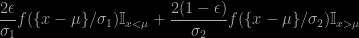
where f is a symmetric density, namely

where

only to show  immediately after that this prior does not allow for a proper posterior, no matter what the sample size is. While the above skewed distribution can always be interpreted as a mixture, being a weighted sum of two terms, it is not strictly speaking a mixture, if only because the “component” can be identified from the observation (depending on which side of μ is stands). The likelihood is therefore a product of simple terms rather than a product of a sum of two terms.

As a solution to this conundrum, the authors consider the alternative of the “independent Jeffreys priors”, which are made of a product of conditional Jeffreys priors, i.e., by computing the Jeffreys prior one parameter at a time with all other parameters considered to be fixed. Which differs from the reference prior, of course, but would have been my second choice as well. Despite criticisms expressed by José Bernardo in the discussion of the paper… The difficulty (in my opinion) resides in the choice (and difficulty) of the parameterisation of the model, since those priors are not parameterisation-invariant. (Xinyi Xu makes the important comment that even those priors incorporate strong if hidden information. Which relates to our earlier discussion with Kaniav Kamari on the “dangers” of prior modelling.)

Although the outcome is puzzling, I remain just slightly sceptical of the income, namely Jeffreys prior and the corresponding Fisher information: the fact that the density involves an indicator function and is thus discontinuous in the location μ at the observation x makes the likelihood function not differentiable and hence the derivation of the Fisher information not strictly valid. Since the indicator part cannot be differentiated. Not that I am seeing the Jeffreys prior as the ultimate grail for non-informative priors, far from it, but there is definitely something specific in the discontinuity in the density. (In connection with the later point, Weiss and Suchard deliver a highly critical commentary on the non-need for reference priors and the preference given to a non-parametric Bayes primary analysis. Maybe making the point towards a greater convergence of the two perspectives, objective Bayes and non-parametric Bayes.)

This paper and the ensuing discussion about the properness of the Jeffreys posterior reminded me of our earliest paper on the topic with Jean Diebolt. Where we used improper priors on location and scale parameters but prohibited allocations (in the Gibbs sampler) that would lead to less than two observations per components, thereby ensuring that the (truncated) posterior was well-defined. (This feature also remained in the Series B paper, submitted at the same time, namely mid-1990, but only published in 1994!)  Larry Wasserman proved ten years later that this truncation led to consistent estimators, but I had not thought about it in very long while. I still like this notion of forcing some (enough) datapoints into each component for an allocation (of the latent indicator variables) to be an acceptable Gibbs move. This is obviously not compatible with the iid representation of a mixture model, but it expresses the requirement that components all have a meaning in terms of the data, namely that all components contributed to generating a part of the data. This translates as a form of weak prior information on how much we trust the model and how meaningful each component is (in opposition to adding meaningless extra-components with almost zero weights or almost identical parameters).

As a marginalia, the insistence in Rubio and Steel’s paper that all observations in the sample be different also reminded me of a discussion I wrote for one of the Valencia proceedings (Valencia 6 in 1998) where Mark presented a paper with Carmen Fernández on this issue of handling duplicated observations modelled by absolutely continuous distributions. (I am afraid my discussion is not worth the $250 price tag given by amazon!)