asymptotically exact inference in likelihood-free models

“We use the intuition that inference corresponds to integrating a density across the manifold corresponding to the set of inputs consistent with the observed outputs.”

Following my earlier post on that paper by Matt Graham and Amos Storkey (University of Edinburgh), I now read through it. The beginning is somewhat unsettling, albeit mildly!, as it starts by mentioning notions like variational auto-encoders, generative adversial nets, and simulator models, by which they mean generative models represented by a (differentiable) function g that essentially turn basic variates with density p into the variates of interest (with intractable density). A setting similar to Meeds’ and Welling’s optimisation Monte Carlo. Another proximity pointed out in the paper is Meeds et al.’s Hamiltonian ABC.

“…the probability of generating simulated data exactly matching the observed data is zero.”

The section on the standard ABC algorithms mentions the fact that ABC MCMC can be (re-)interpreted as a pseudo-marginal MCMC, albeit one targeting the ABC posterior instead of the original posterior. The starting point of the paper is the above quote, which echoes a conversation I had with Gabriel Stolz a few weeks ago, when he presented me his free energy method and when I could not see how to connect it with ABC, because having an exact match seemed to cancel the appeal of ABC, all parameter simulations then producing an exact match under the right constraint. However, the paper maintains this can be done, by looking at the joint distribution of the parameters, latent variables, and observables. Under the implicit restriction imposed by keeping the observables constant. Which defines a manifold. The mathematical validation is achieved by designing the density over this manifold, which looks like

if the constraint can be rewritten as g⁰(u)=0. (This actually follows from a 2013 paper by Diaconis, Holmes, and Shahshahani.) In the paper, the simulation is conducted by Hamiltonian Monte Carlo (HMC), the leapfrog steps consisting of an unconstrained move followed by a projection onto the manifold. This however sounds somewhat intense in that it involves a quasi-Newton resolution at each step. I also find it surprising that this projection step does not jeopardise the stationary distribution of the process, as the argument found therein about the approximation of the approximation is not particularly deep. But the main thing that remains unclear to me after reading the paper is how the constraint that the pseudo-data be equal to the observable data can be turned into a closed form condition like g⁰(u)=0. As mentioned above, the authors assume a generative model based on uniform (or other simple) random inputs but this representation seems impossible to achieve in reasonably complex settings.

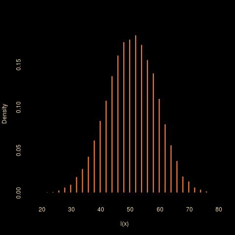
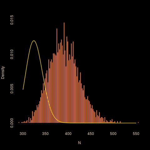
exact ABC

Minh-Ngoc Tran and Robert Kohn have devised an “exact” ABC algorithm. They claim therein to remove the error due to the non-zero tolerance by using an unbiased estimator of the likelihood. Most interestingly, they start from the debiasing technique of Rhee and Glynn [also at the basis of the Russian roulette]. Which sums up as using a telescoping formula on a sequence of converging biased estimates. And cutting the infinite sum with a stopping rule.

“Our article proposes an ABC algorithm to estimate [the observed likelihood] that completely removes the error due to [the ABC] approximation…”

The sequence of biased but converging approximations is associated with a sequence of decreasing tolerances. The corresponding sequence of weights that determines the truncation in the series is connected to the decrease in the bias in an implicit manner for all realistic settings. Although Theorem 1 produces conditions on the ABC kernel and the sequence of tolerances and pseudo-sample sizes that guarantee unbiasedness and finite variance of the likelihood estimate. For a geometric stopping rule with rejection probability p, both tolerance and pseudo-sample size decrease as a power of p. As a side product the method also returns an unbiased estimate of the evidence. The overall difficulty I have with the approach is the dependence on the stopping rule and its calibration, and the resulting impact on the computing time of the likelihood estimate. When this estimate is used in a pseudo-marginal scheme à la Andrieu and Roberts (2009), I fear this requires new pseudo-samples at each iteration of the Metropolis-Hastings algorithm, which then becomes prohibitively expensive. Later today, Mark Girolami pointed out to me that Anne-Marie Lyne [one of the authors of the Russian roulette paper] also considered this exact approach in her thesis and concluded at an infinite computing time.

likelihood-free inference in high-dimensional models

“…for a general linear model (GLM), a single linear function is a sufficient statistic for each associated parameter…”

The recently arXived paper “Likelihood-free inference in high-dimensional models“, by Kousathanas et al. (July 2015), proposes an ABC resolution of the dimensionality curse [when the dimension of the parameter and of the corresponding summary statistics] by turning Gibbs-like and by using a component-by-component ABC-MCMC update that allows for low dimensional statistics. In the (rare) event there exists a conditional sufficient statistic for each component of the parameter vector, the approach is just as justified as when using a generic ABC-Gibbs method based on the whole data. Otherwise, that is, when using a non-sufficient estimator of the corresponding component (as, e.g., in a generalised [not general!] linear model), the approach is less coherent as there is no joint target associated with the Gibbs moves. One may therefore wonder at the convergence properties of the resulting algorithm. The only safe case [in dimension 2] is when one of the restricted conditionals does not depend on the other parameter. Note also that each Gibbs step a priori requires the simulation of a new pseudo-dataset, which may be a major imposition on computing time. And that setting the tolerance for each parameter is a delicate calibration issue because in principle the tolerance should depend on the other component values.

the Flatland paradox [#2]

Another trip in the métro today (to work with Pierre Jacob and Lawrence Murray in a Paris Anticafé!, as the University was closed) led me to infer—warning!, this is not the exact distribution!—the distribution of x, namely

since a path x of length l(x) will corresponds to N draws if N-l(x) is an even integer 2p and p undistinguishable annihilations in 4 possible directions have to be distributed over l(x)+1 possible locations, with Feller’s number of distinguishable distributions as a result. With a prior π(N)=1/N on N, hence on p, the posterior on p is given by

Now, given N and  x, the probability of no annihilation on the last round is 1 when l(x)=N and in general

which can be integrated against the posterior. The numerical expectation is represented for a range of values of l(x) in the above graph. Interestingly, the posterior probability is constant for l(x) large  and equal to 0.8125 under a flat prior over N.

Getting back to Pierre Druilhet’s approach, he sets a flat prior on the length of the path θ and from there derives that the probability of annihilation is about 3/4. However, “the uniform prior on the paths of lengths lower or equal to M” used for this derivation which gives a probability of length l proportional to 3^l is quite different from the distribution of l(θ) given a number of draws N. Which as shown above looks much more like a Binomial B(N,1/2).

However, being not quite certain about the reasoning involving Fieller’s trick, I ran an ABC experiment under a flat prior restricted to (l(x),4l(x)) and got the above, where the histogram is for a posterior sample associated with l(x)=195 and the gold curve is the potential posterior. Since ABC is exact in this case (i.e., I only picked N’s for which l(x)=195), ABC is not to blame for the discrepancy! I asked about the distribution on Stack Exchange maths forum (and a few colleagues here as well) but got no reply so far… Here is the R code that goes with the ABC implementation:

#observation:
elo=195
#ABC version
T=1e6
el=rep(NA,T)
N=sample(elo:(4*elo),T,rep=TRUE)
for (t in 1:T){
#generate a path
  paz=sample(c(-(1:2),1:2),N[t],rep=TRUE)
#eliminate U-turns
  uturn=paz[-N[t]]==-paz[-1]
  while (sum(uturn>0)){
    uturn[-1]=uturn[-1]*(1-
              uturn[-(length(paz)-1)])
    uturn=c((1:(length(paz)-1))[uturn==1],
            (2:length(paz))[uturn==1])
    paz=paz[-uturn]
    uturn=paz[-length(paz)]==-paz[-1]
    }
  el[t]=length(paz)}
#subsample to get exact posterior
poster=N[abs(el-elo)==0]