The [errors in the] error of truth [book review]

OUP sent me this book, The error of truth by Steven Osterling, for review. It is a story about the “astonishing” development of quantitative thinking in the past two centuries. Unfortunately, I found it to be one of the worst books I have read on the history of sciences…

To start with the rather obvious part, I find the scholarship behind the book quite shoddy as the author continuously brings in items of historical tidbits to support his overall narrative and sometimes fills gaps on his own. It often feels like the material comes from Wikipedia, despite expressing a critical view of the on-line encyclopedia. The [long] quote below is presumably the most shocking historical blunder, as the terror era marks the climax of the French Revolution, rather than the last fight of the French monarchy. Robespierre was the head of the Jacobins, the most radical revolutionaries at the time, and one of the Assembly members who voted for the execution of Louis XIV, which took place before the Terror. And later started to eliminate his political opponents, until he found himself on the guillotine!

“The monarchy fought back with almost unimaginable savagery. They ordered French troops to carry out a bloody campaign in which many thousands of protesters were killed. Any peasant even remotely suspected of not supporting the government was brutally killed by the soldiers; many were shot at point-blank range. The crackdown’s most intense period was a horrific ten-month Reign of Terror (“la Terreur”) during which the government guillotined untold masses (some estimates are as high as 5,000) of its own citizens as a means to control them. One of the architects of the Reign of Terror was Maximilien Robespierre, a French nobleman and lifelong politician. He explained the government’s slaughter in unbelievable terms, as “justified terror . . . [and] an emanation of virtue” (quoted in Linton 2006). Slowly, however, over the next few years, the people gained control. In the end, many nobles, including King Louis XVI and his wife Marie-Antoinette, were themselves executed by guillotining”

Obviously, this absolute misinterpretation does not matter (very) much for the (hi)story of quantification (and uncertainty assessment), but it demonstrates a lack of expertise of the author. And sap whatever trust one could have in new details he brings to light (life?). As for instance when stating

“Bayes did a lot of his developmental work while tutoring students in local pubs. He was a respected teacher. Taking advantage of his immediate resources (in his circumstance, a billiard table), he taught his theorem to many.”

which does not sound very plausible. I never heard that Bayes had students  or went to pubs or exposed his result to many before its posthumous publication… Or when Voltaire (who died in 1778) is considered as seventeenth-century precursor of the Enlightenment. Or when John Graunt, true member of the Royal Society, is given as a member of the Académie des Sciences. Or when Quetelet is presented as French and as a student of Laplace.

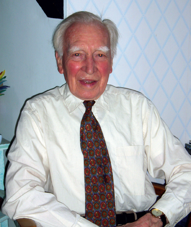
The maths explanations are also puzzling, from the law of large numbers illustrated by six observations, and wrongly expressed (p.54) as

to  the Saint-Petersbourg paradox being seen as inverse probability, to a botched description of the central limit theorem  (p.59), including the meaningless equation (p.60)

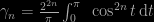
to de Moivre‘s theorem being given as Taylor’s expansion

and as his derivation of the concept of variance, to another botched depiction of the difference between Bayesian and frequentist statistics, incl. the usual horror

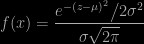
to independence being presented as a non-linear relation (p.111), to the conspicuous absence of Pythagoras in the regression chapter, to attributing to Gauss the concept of a probability density (when Simpson, Bayes, Laplace used it as well), to another highly confusing verbal explanation of densities, including a potential confusion between different representations of a distribution (Fig. 9.6) and the existence of distributions other than the Gaussian distribution, to another error in writing the Gaussian pdf (p.157),

to yet another error in the item response probability (p.301), and.. to completely missing the distinction between the map and the territory, i.e., the probabilistic model and the real world (“Truth”), which may be the most important shortcoming of the book.

The style is somewhat heavy, with many repetitions about the greatness of the characters involved in the story, and some degree of license in bringing them within the narrative of the book. The historical determinism of this narrative is indeed strong, with a tendency to link characters more than they were, and to make them greater than life. Which is a usual drawback of such books, along with the profuse apologies for presenting a few mathematical formulas!

The overall presentation further has a Victorian and conservative flavour in its adoration of great names, an almost exclusive centering on Western Europe, a patriarchal tone (“It was common for them to assist their husbands in some way or another”, p.44; Marie Curie “agreed to the marriage, believing it would help her keep her laboratory position”, p.283), a defense of the empowerment allowed by the Industrial Revolution and of the positive sides of colonialism and of the Western expansion of the USA, including the invention of Coca Cola as a landmark in the march to Progress!, to the fall of the (communist) Eastern Block being attributed to Ronald Reagan, Karol Wojtyła, and Margaret Thatcher, to the Bell Curve being written by respected professors with solid scholarship, if controversial, to missing the Ottoman Enlightenment and being particularly disparaging about the Middle East, to dismissing Galton’s eugenism as a later year misguided enthusiasm (and side-stepping the issue of Pearson’s and Fisher’s eugenic views),

Another recurrent if minor problem is the poor recording of dates and years when introducing an event or a new character. And the quotes referring to the current edition or translation instead of the original year as, e.g., Bernoulli (1954). Or even better!, Bayes and Price (1963).

[Disclaimer about potential self-plagiarism: this post or an edited version will eventually appear in my Book Review section in CHANCE.]

a Simpson paradox of sorts

The riddle from The Riddler this week is about finding an undirected graph with N nodes and no isolated node such that the number of nodes with more connections than the average of their neighbours is maximal. A representation of a connected graph is through a matrix X of zeros and ones, on which one can spot the nodes satisfying the above condition as the positive entries of the vector (X1)^2-(X^21), if 1 denotes the vector of ones. I thus wrote an R code aiming at optimising this target

targe <- function(F){
  sum(F%*%F%*%rep(1,N)/(F%*%rep(1,N))^2<1)}

by mere simulated annealing:

rate <- function(N){ 
# generate matrix F
# 1. no single 
F=matrix(0,N,N) 
F[sample(2:N,1),1]=1 
F[1,]=F[,1] 
for (i in 2:(N-1)){ 
if (sum(F[,i])==0) 
F[sample((i+1):N,1),i]=1 
F[i,]=F[,i]} 
if (sum(F[,N])==0) 
F[sample(1:(N-1),1),N]=1 
F[N,]=F[,N] 
# 2. more connections 
F[lower.tri(F)]=F[lower.tri(F)]+
  sample(0:1,N*(N-1)/2,rep=TRUE,prob=c(N,1)) 
F[F>1]=1
F[upper.tri(F)]=t(F)[upper.tri(t(F))]
#simulated annealing
T=1e4
temp=N
targo=targe(F)
for (t in 1:T){
  #1. local proposal
  nod=sample(1:N,2)
  prop=F
  prop[nod[1],nod[2]]=prop[nod[2],nod[1]]=
     1-prop[nod[1],nod[2]]
  while (min(prop%*%rep(1,N))==0){
    nod=sample(1:N,2)
    prop=F
    prop[nod[1],nod[2]]=prop[nod[2],nod[1]]=
     1-prop[nod[1],nod[2]]}
  target=targe(prop)
  if (log(runif(1))*temp<target-targo){ 
    F=prop;targo=target} 
#2. global proposal 
  prop=F prop[lower.tri(prop)]=F[lower.tri(prop)]+
   sample(c(0,1),N*(N-1)/2,rep=TRUE,prob=c(N,1)) 
prop[prop>1]=1
  prop[upper.tri(prop)]=t(prop)[upper.tri(t(prop))]
  target=targe(prop)
  if (log(runif(1))*temp<target-targo){
      F=prop;targo=target}
   temp=temp*.999
   }
return(F)}

This code returns quite consistently (modulo the simulated annealing uncertainty, which grows with N) the answer N-2 as the number of entries above average! Which is rather surprising in a Simpson-like manner since all entries but two are above average. (Incidentally, I found out that Edward Simpson recently wrote a paper in Significance about the Simpson-Yule paradox and him being a member of the Bletchley Park Enigma team. I must have missed out the connection with the Simpson paradox when reading the paper in the first place…)