Bertrand’s paradox [re]solved?

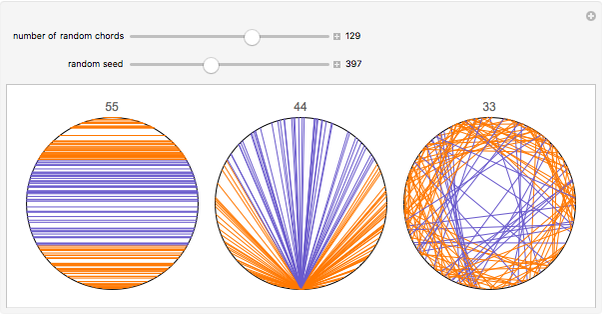
On the plane back from Vancouver, I read Bertrand’s Paradox Resolution and Its Implications for the Bing–Fisher Problem by Richard A. Chechile [who had pointed out his paper to me] In this paper, Chechile considers the Bayesian connections/sequences of Betrand’s paradox, as he sees it Bertrand’s different solutions/paradox to be

“designed to illustrate his dissatisfaction with the Bayes and Laplace use of a probability distribution to represent an unknown parameter that can have any continuous value”

and proposes to “resolve” this paradox, which imho is neither a paradox nor in need of a resolution!, as I see it more like a reflection on the importance of sigma algebras and measure theory. The uniform distribution (behind the “random” chord) is not a uniquely specified concept, just like the maximum entropy distribution is relative to the dominating measure. When arguing that

“Such a definition [based on any possible distribution of a stochastic chord] would yield a random variable, but this weak sense of the word random is not satisfactory, because there is an infinite number of stochastic processes that can be defined to yield a probability distribution of chord lengths.”

the author is simply restating that infinite collection of dominating measures.  But imho he is somewhat missing this point when defining Shannon`s entropy by resorting to a discrete version. And when adopting a uniform measure on the chord as a reference (Section 3.2, on The Importance of a Dominant Metric Representation). While the probability P(L>1) is invariant under any increasing transform of L (and 1)… This amounts to arguing for a favourite parameterisation in constructing  a reference prior (Section 4, where Jeffreys prior is also dismissed for not being at maximum entropy). The ensuing discussion as to why the three solutions of Bertrand’s are not valid (Section 2.2) is thus most curious to me since they all are implementable/practical ways of producing stochastic chords. I find it rather amusing that one returns to the quest for the ideal priori distribution Bayesians were so fiercely debating at the turn of the previous century. And non-Bayesians were all too happy to exploit when arguing against this approach.

Bertrand’s tartine

A riddle from The Riddler on cutting a square (toast) into two parts and keeping at least 25% of the surface on each part while avoiding Bertrand’s paradox. By defining the random cut as generated by two uniform draws over the periphery of the square. Meaning that ¼ of the draws are on the same side, ½ on adjacent sides and again ¼ on opposite sides. Meaning one has to compute

P(UV>½)= ½(1-log(2))

and

P(½(U+V)∈(¼,¾))= ¾

Resulting in a probability of 0.2642 (checked by simulation)

Bertrand-Borel debate

On her blog, Deborah Mayo briefly mentioned the Bertrand-Borel debate on the (in)feasibility of hypothesis testing, as reported [and translated] by Erich Lehmann. A first interesting feature is that both [starting with] B mathematicians discuss the probability of causes in the Bayesian spirit of Laplace. With Bertrand considering that the prior probabilities of the different causes are impossible to set and then moving all the way to dismiss the use of probability theory in this setting, nipping the p-values in the bud..! And Borel being rather vague about the solution probability theory has to provide. As stressed by Lehmann.

“The Pleiades appear closer to each other than one would naturally expect. This statement deserves thinking about; but when one wants to translate the phenomenon into numbers, the necessary ingredients are lacking. In order to make the vague idea of closeness more precise, should we look for the smallest circle that contains the group? the largest of the angular distances? the sum of squares of all the distances? the area of the spherical polygon of which some of the stars are the vertices and which contains the others in its interior? Each of these quantities is smaller for the group of the Pleiades than seems plausible. Which of them should provide the measure of implausibility? If three of the stars form an equilateral triangle, do we have to add this circumstance, which is certainly very unlikely apriori, to those that point to a cause?” Joseph Bertrand (p.166)

 

“But whatever objection one can raise from a logical point of view cannot prevent the preceding question from arising in many situations: the theory of probability cannot refuse to examine it and to give an answer; the precision of the response will naturally be limited by the lack of precision in the question; but to refuse to answer under the pretext that the answer cannot be absolutely precise, is to place oneself on purely abstract grounds and to misunderstand the essential nature of the application of mathematics.” Emile Borel (Chapter 4)

Another highly interesting objection of Bertrand is somewhat linked with his conditioning paradox, namely that the density of the observed unlikely event depends on the choice of the statistic that is used to calibrate the unlikeliness, which makes complete sense in that the information contained in each of these statistics and the resulting probability or likelihood differ to an arbitrary extend, that there are few cases (monotone likelihood ratio) where the choice can be made, and that Bayes factors share the same drawback if they do not condition upon the entire sample. In which case there is no selection of “circonstances remarquables”. Or of uniformly most powerful tests.

Le Monde puzzle [#1024]

The penultimate and appropriately somewhat Monty Hallesque Le Monde mathematical puzzle of the competition!

A dresser with 5×5 drawers contains a single object in one of the 25 drawers. A player opens a drawer at random and, after each choice, the object moves at random to a drawer adjacent to its current location and the drawer chosen by the player remains open. What is the maximum number of drawers one need to open to find the object?

In a dresser with 9 drawers in a line, containing again a single object, the player opens drawers one at a time, after which the open drawer is closed and the object moves to one of the drawers adjacent to its current location. What is the maximum number of drawers one need to open to find the object?

For the first question, setting a pattern of exploration and, given this pattern, simulating a random walk trying to avoid the said pattern as long as possible is feasible, returning a maximum number of steps over many random walks [and hence a lower bound on the true maximum]. As in the following code

sefavyd=function(pater=seq(1,49,2)%%25+1){
  fild=matrix(0,5,5)
  m=pater[1];i=fild[m]=1
  t=sample((1:25)[-m],1)
  nomove=FALSE
  while (!nomove){
   i=i+1
   m=pater[i];fild[m]=1
   if (t==m){ nomove=TRUE}else{
   muv=NULL
   if ((t-1)%%5>0) muv=c(muv,t-1)
   if (t%%5>0) muv=c(muv,t+1)
   if ((t-1)%/%5>0) muv=c(muv,t-5)
   if (t%/%5<4) muv=c(muv,t+5)
   muv=muv[fild[muv]==0]
   nomove=(length(muv)==0)
   if (!nomove) t=sample(rep(muv,2),1)}
  }
  return(i)}

But a direct reasoning starts from the observation that, while two adjacent drawers are not opened, a random walk can, with non-zero probability, switch indefinitely between both drawers. Hence, a sure recovery of the object requires opening one drawer out of two. The minimal number of drawers to open on a 5×5 dresser is 2+3+2+3+2=12. Since in 12 steps, those drawers are all open, spotting the object may require up to 13 steps.

For the second case, unless I [again!] misread the question, whatever pattern one picks for the exploration, there is always a non-zero probability to avoid discovery after an arbitrary number of steps. The [wrong!] answer is thus infinity. To cross-check this reasoning, I wrote the following R code that mimics a random pattern of exploration, associated by an opportunistic random walk that avoids discovery whenever possible (even with very low probability) bu pushing the object towards the centre,

drawl=function(){
  i=1;t=5;nomove=FALSE
  m=sample((1:9)[-t],1)
  while (!nomove){
    nextm=sample((1:9),1)
    muv=c(t-1,t+1)
    muv=muv[(muv>0)&(muv<10)&(muv!=nextm)] 
    nomove=(length(muv)==0)||(i>1e6)
    if (!nomove) t=sample(rep(muv,2),1,
              prob=1/(5.5-rep(muv,2))^4)
    i=i+1}
  return(i)}

which returns unlimited values on repeated runs. However, I was wrong and the R code unable to dismiss my a priori!, as later discussions with Robin and Julien at Paris-Dauphine exhibited ways of terminating the random walk in 18, then 15, then 14 steps! The idea was to push the target to one of the endpoints because it would then have no option but turning back: an opening pattern like 2, 3, 4, 5, 6, 7, 8, 8 would take care of a hidden object starting in an even drawer, while the following 7, 6, 5, 4, 3, 2 openings would terminate any random path starting from an odd drawer. To double check:

grawl=function(){
  len=0;muvz=c(3:8,8:1)
  for (t in 1:9){
    i=1;m=muvz[i];nomove=(t==m)
    while (!nomove){
     i=i+1;m=muvz[i];muv=c(t-1,t+1)
     muv=muv[(muv>0)&(muv<10)&(muv!=m)]
     nomove=(length(muv)==0)
     if (!nomove)
      t=sample(rep(muv,2),1)}
    len=max(len,i)}
  return(len)}

produces the value 14.

what makes variables randoms [book review]

When the goal of a book is to make measure theoretic probability available to applied researchers for conducting their research, I cannot but applaud! Peter Veazie’s goal of writing “a brief text that provides a basic conceptual introduction to measure theory” (p.4) is hence most commendable. Before reading What makes variables random, I was uncertain how this could be achieved with a limited calculus background, given the difficulties met by our third year maths students. After reading the book, I am even less certain this is feasible!

“…it is the data generating process that makes the variables random and not the data.”

Chapter 2 is about basic notions of set theory. Chapter 3 defines measurable sets and measurable functions and integrals against a given measure μ as

which I find particularly unnatural compared with the definition through simple functions (esp. because it does not tell how to handle 0x∞). The ensuing discussion shows the limitation of the exercise in that the definition is only explained for finite sets (since the notion of a partition achieving the supremum on page 29 is otherwise meaningless). A generic problem with the book, in that most examples in the probability section relate to discrete settings (see the discussion of the power set p.66). I also did not see a justification as to why measurable functions enjoy well-defined integrals in the above sense. All in all, to see less than ten pages allocated to measure theory per se is rather staggering! For instance,

does not appear to be defined at all.

“…the mathematical probability theory underlying our analyses is just mathematics…”

Chapter 4 moves to probability measures. It distinguishes between objective (or frequentist) and subjective measures, which is of course open to diverse interpretations. And the definition of a conditional measure is the traditional one, conditional on a set rather than on a σ-algebra. Surprisingly as this is in my opinion one major reason for using measures in probability theory. And avoids unpleasant issues such as Bertrand’s paradox. While random variables are defined in the standard sense of real valued measurable functions, I did not see a definition of a continuous random variables or of the Lebesgue measure. And there are only a few lines (p.48) about the notion of expectation, which is so central to measure-theoretic probability as to provide a way of entry into measure theory! Progressing further, the σ-algebra induced by a random variable is defined as a partition (p.52), a particularly obscure notion for continuous rv’s. When the conditional density of one random variable given the realisation of another is finally introduced (p.63), as an expectation reconciling with the set-wise definition of conditional probabilities, it is in a fairly convoluted way that I fear will scare newcomers out of their wit. Since it relies on a sequence of nested sets with positive measure, implying an underlying topology and the like, which somewhat shows the impossibility of the overall task…

“In the Bayesian analysis, the likelihood provides meaning to the posterior.”

Statistics is hurriedly introduced in a short section at the end of Chapter 4, assuming the notion of likelihood is already known by the readers. But nitpicking (p.65) at the representation of the terms in the log-likelihood as depending on an unspecified parameter value θ [not to be confused with the data-generating value of θ, which does not appear clearly in this section]. Section that manages to include arcane remarks distinguishing maximum likelihood estimation from Bayesian analysis, all this within a page! (Nowhere is the Bayesian perspective clearly defined.)

“We should no more perform an analysis clustered by state than we would cluster by age, income, or other random variable.”

The last part of the book is about probabilistic models, drawing a distinction between data generating process models and data models (p.89), by which the author means the hypothesised probabilistic model versus the empirical or bootstrap distribution. An interesting way to relate to the main thread, except that the convergence of the data distribution to the data generating process model cannot be established at this level. And hence that the very nature of bootstrap may be lost on the reader. A second and final chapter covers some common or vexing problems and the author’s approach to them. Revolving around standard errors, fixed and random effects. The distinction between standard deviation (“a mathematical property of a probability distribution”) and standard error (“representation of variation due to a data generating process”) that is followed for several pages seems to boil down to a possible (and likely) model mis-specification. The chapter also contains an extensive discussion of notations, like indexes (or indicators), which seems a strange focus esp. at this location in the book. Over 15 pages! (Furthermore, I find quite confusing that a set of indices is denoted there by the double barred I, usually employed for the indicator function.)

“…the reader will probably observe the conspicuous absence of a time-honoured topic in calculus courses, the “Riemann integral”… Only the stubborn conservatism of academic tradition could freeze it into a regular part of the curriculum, long after it had outlived its historical importance.” Jean Dieudonné, Foundations of Modern Analysis

In conclusion, I do not see the point of this book, from its insistence on measure theory that never concretises for lack of mathematical material to an absence of convincing examples as to why this is useful for the applied researcher, to the intended audience which is expected to already quite a lot about probability and statistics, to a final meandering around linear models that seems at odds with the remainder of What makes variables random, without providing an answer to this question. Or to the more relevant one of why Lebesgue integration is preferable to Riemann integration. (Not that there does not exist convincing replies to this question!)