taking advantage of the constant

A question from X validated had enough appeal for me to procrastinate about it for ½ an hour: what difference does it make [for simulation purposes] that a target density is properly normalised? In the continuous case, I do not see much to exploit about this knowledge, apart from the value potentially leading to a control variate (in a Gelfand and Dey 1996 spirit) and possibly to a stopping rule (by checking that the portion of the space visited so far has mass close to one, but this is more delicate than it sounds).

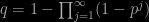
In a (possibly infinite) countable setting, it seems to me one gain (?) is that approximating expectations by Monte Carlo no longer requires iid simulations in the sense that once visited,  atoms need not be visited again. Self-avoiding random walks and their generalisations thus appear as a natural substitute for MC(MC) methods in this setting, provided finding unexplored atoms proves manageable. For instance, a stopping rule is always available, namely that the cumulated weight of the visited fraction of the space is close enough to one. The above picture shows a toy example on a 500 x 500 grid with 0.1% of the mass remaining at the almost invisible white dots. (In my experiment, neighbours for the random exploration were chosen at random over the grid, as I assumed no global information was available about the repartition over the grid either of mass function or of the function whose expectation was seeked.)

practical PDMP

While in Warwick, last month, I attended a reading group on PDMPs where Filippo Pagani talked about practical PDMP, connected with a recent arXival by Bertazzi, Bierkens and Dobson. The central question when implementing PDMP is to find a realistic way of solving

to decide on the stopping time (when the process ceases to be deterministic). The usual approach is to use Poisson thinning by finding an upper bound on λ, but this is either difficult or potentially inefficient (and sometimes both).

“finding a sharp bound M(s) [for Poisson thinning] can be an extremely challenging problem in most practical settings (…) In order to overcome this problem, we introduce discretisation schemes for PDMPs which make their
approximate simulation possible.”

Some of the solutions proposed in Bertazzi et al. are relying on

1. using a frozen (fixed) λ
2. discretising time and the integral (first order scheme)
3. allowing for more than a jump over a time interval (higher order schemes)
4. going through control variates (when gradient is Lipschitz and Hessian bounded, with known constants) as it produces a linear rate λ
5. subsampling (at least for Zig Zag)

with theoretical guarantees that the approximations are convergent, as the time step goes to zero. They (almost obviously) remain model dependent solutions (with illustrations for the Zig Zag and bouncy particle versions), with little worse case scenarios, but this is an extended investigation into making PDMPs more manageable!

back to the Bernoulli factory

“The results show that the proposed algorithm is asymptotically optimal for the mentioned subclass of functions, in the sense that for any other fast algorithm E[N] grows at least as fast with p.”

Murray Pollock (Warwick U. for a wee more days!) pointed out to me this paper of Luis Mendo on a Bernoulli factory algorithm that estimates functions [of p] that can be expressed as power series [of p]. Essentially functions f(p) such that f(0)=0 and f(1)=1. The big difference with earlier algorithms, as far as I can tell, is that the approach involves a randomised stopping rule that involves, on top of the unlimited sequence of Bernoulli B(p) variates a second sequence of Uniform variates, which sounds to me like a change of paradigm, given the much higher degree of freedom brought by Uniform variates (as opposed to Bernoulli variates with an unknown value of p). Although there exists a non-randomised version in the paper. The proposed algorithm is as follows, using a sequence of d’s issued from the power series coefficients:

1. Set i=1.
2. Take one input X[i].
3. Produce U[i] uniform on (0,1). Let V[i]=1 if U[i]<d[i] and V[i]=0 otherwise.
If V[i] or X[i] are equal to 1, output X[i] and finish.
Else increase i and go back to step2.

As the author mentions, this happens to be a particular case of the reverse-time martingale approach of Łatuszynski, Kosmidis, Papaspiliopoulos and Roberts (Warwick connection as well!). With an average number of steps equal to f(p)/p, surprisingly simple, and somewhat of an optimal rate. While the functions f(p) are somewhat restricted, this is nice work

revisiting the Gelman-Rubin diagnostic

Just before Xmas, Dootika Vats (Warwick) and Christina Knudson arXived a paper on a re-evaluation of the ultra-popular 1992 Gelman and Rubin MCMC convergence diagnostic. Which compares within-variance and between-variance on parallel chains started from hopefully dispersed initial values. Or equivalently an under-estimating and an over-estimating estimate of the MCMC average. In this paper, the authors take advantage of the variance estimators developed by Galin Jones, James Flegal, Dootika Vats and co-authors, which are batch mean estimators consistently estimating the asymptotic variance. They also discuss the choice of a cut-off on the ratio R of variance estimates, i.e., how close to one need it be? By relating R to the effective sample size (for which we also have reservations), which gives another way of calibrating the cut-off. The main conclusion of the study is that the recommended 1.1 bound is too large for a reasonable proximity to the true value of the Bayes estimator (Disclaimer: The above ABCruise header is unrelated with the paper, apart from its use of the Titanic dataset!)

In fact, I have other difficulties than setting the cut-off point with the original scheme as a way to assess MCMC convergence or lack thereof, among which

1. its dependence on the parameterisation of the chain and on the estimation of a specific target function
2. its dependence on the starting distribution which makes the time to convergence not absolutely meaningful
3. the confusion between getting to stationarity and exploring the whole target
4. its missing the option to resort to subsampling schemes to attain pseudo-independence or scale time to convergence (albeit see 3. above)
5. a potential bias brought by the stopping rule.

a funny mistake

While watching the early morning activity in Tofino inlet from my rental desk, I was looking at a recent fivethirthyeight Riddle, which consisted in finding the probability of stopping a coin game which rule was to wait for the n consecutive heads if (n-1) consecutive heads had failed to happen when requested, which is

p+(1-p)p²+(1-p)(1-p²)p³+…

or

While the above can write as

or

hence suggesting

the answer is (obviously) false and the mistake in separating the series into a difference of series is that both terms are infinite. The correct answer is actually

which is Euler’s function. Maybe nonstandard analysis can apply to go directly from the difference of the infinite series to the answer!