one bridge further

Jackie Wong, Jon Forster (Warwick) and Peter Smith have just published a paper in Statistics & Computing on bridge sampling bias and improvement by splitting.

“… known to be asymptotically unbiased, bridge sampling technique produces biased estimates in practical usage for small to moderate sample sizes (…) the estimator yields positive bias that worsens with increasing distance between the two distributions. The second type of bias arises when the approximation density is determined from the posterior samples using the method of moments, resulting in a systematic underestimation of the normalizing constant.”

Recall that bridge sampling is based on a double trick with two samples x and y from two (unnormalised) densities f and g that are interverted in a ratio

of unbiased estimators of the inverse normalising constants. Hence biased. The more the less similar these two densities are. Special cases for ω include importance sampling [unbiased] and reciprocal importance sampling. Since the optimal version of the bridge weight ω is the inverse of the mixture of f and g, it makes me wonder at the performance of using both samples top and bottom, since as an aggregated sample, they also come from the mixture, as in Owen & Zhou (2000) multiple importance sampler. However, a quick try with a positive Normal versus an Exponential with rate 2 does not show an improvement in using both samples top and bottom (even when using the perfectly normalised versions)

morc=(sum(f(y)/(nx*dnorm(y)+ny*dexp(y,2)))+
            sum(f(x)/(nx*dnorm(x)+ny*dexp(x,2))))/(
  sum(g(x)/(nx*dnorm(x)+ny*dexp(x,2)))+
         sum(g(y)/(nx*dnorm(y)+ny*dexp(y,2))))

at least in terms of bias… Surprisingly (!) the bias almost vanishes for very different samples sizes either in favour of f or in favour of g. This may be a form of genuine defensive sampling, who knows?! At the very least, this ensures a finite variance for all weights. (The splitting approach introduced in the paper is a natural solution to create independence between the first sample and the second density. This reminded me of our two parallel chains in AMIS.)

bridgesampling [R package]

Quentin F. Gronau, Henrik Singmann and Eric-Jan Wagenmakers have arXived a detailed documentation about their bridgesampling R package. (No wonder that researchers from Amsterdam favour bridge sampling!) [The package relates to a [52 pages] tutorial on bridge sampling by Gronau et al. that I will hopefully comment soon.] The bridge sampling methodology for marginal likelihood approximation requires two Monte Carlo samples for a ratio of two integrals. A nice twist in this approach is to use a dummy integral that is already available, with respect to a probability density that is an approximation to the exact posterior. This means avoiding the difficulties with bridge sampling of bridging two different parameter spaces, in possibly different dimensions, with potentially very little overlap between the posterior distributions. The substitute probability density is chosen as Normal or warped Normal, rather than a t which would provide more stability in my opinion. The bridgesampling package also provides an error evaluation for the approximation, although based on spectral estimates derived from the coda package. The remainder of the document exhibits how the package can be used in conjunction with either JAGS or Stan. And concludes with the following words of caution:

“It should also be kept in mind that there may be cases in which the bridge sampling procedure may not be the ideal choice for conducting Bayesian model comparisons. For instance, when the models are nested it might be faster and easier to use the Savage-Dickey density ratio (Dickey and Lientz 1970; Wagenmakers et al. 2010). Another example is when the comparison of interest concerns a very large model space, and a separate bridge sampling based computation of marginal likelihoods may take too much time. In this scenario, Reversible Jump MCMC (Green 1995) may be more appropriate.”

warp-U bridge sampling

[I wrote this set of comments right after MCqMC 2016 on a preliminary version of the paper so mileage may vary in terms of the adequation to the current version!]

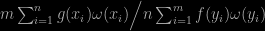
In warp-U bridge sampling, newly arXived and first presented at MCqMC 16, Xiao-Li Meng continues (in collaboration with Lahzi Wang) his exploration of bridge sampling techniques towards improving the estimation of normalising constants and ratios thereof. The bridge sampling estimator of Meng and Wong (1996) is an harmonic mean importance sampler that requires iterations as it depends on the ratio of interest. Given that the normalising constant of a density does not depend on the chosen parameterisation in the sense that the Jacobian transform preserves this constant, a degree of freedom is in the choice of the parameterisation. This is the idea behind warp transformations. The initial version of Meng and Schilling (2002) used location-scale transforms, while the warp-U solution goes for a multiple location-scale transform that can be seen as based on a location-scale mixture representation of the target. With K components. This approach can also be seen as a sort of artificial reversible jump algorithm when one model is fully known. A strategy Nicolas and I also proposed in our nested sampling Biometrika paper.

Once such a mixture approximation is obtained. each and every component of the mixture can be turned into the standard version of the location-scale family by the appropriate location-scale transform. Since the component index k is unknown for a given X, they call this transform a random transform, which I find somewhat more confusing that helpful. The conditional distribution of the index given the observable x is well-known for mixtures and it is used here to weight the component-wise location-scale transforms of the original distribution p into something that looks rather similar to the standard version of the location-scale family. If no mode has been forgotten by the mixture. The simulations from the original p are then rescaled by one of those transforms, which index k is picked according to the conditional distribution. As explained later to me by XL, the random[ness] in the picture is due to the inclusion of a random ± sign. Still, in the notation introduced in (13), I do not get how the distribution Þ [sorry for using different symbols, I cannot render a tilde on a p] is defined since both ψ and W are random. Is it the marginal? In which case it would read as a weighted average of rescaled versions of p. I have the same problem with Theorem 1 in that I do not understand how one equates Þ with the joint distribution.

Equation (21) is much more illuminating (I find) than the previous explanation in that it exposes the fact that the principle is one of aiming at a new distribution for both the target and the importance function, with hopes that the fit will get better. It could have been better to avoid the notion of random transform, then, but this is mostly a matter of conveying the notion.

On more specifics points (or minutiae), the unboundedness of the likelihood is rarely if ever a problem when using EM. An alternative to the multiple start EM proposal would then be to get sequential and estimate the mixture in a sequential manner, only adding a component when it seems worth it. See eg Chopin and Pelgrin (2004) and Chopin (2007). This could also help with the bias mentioned therein since only a (tiny?) fraction of the data would be used. And the number of components K has an impact on the accuracy of the approximation, as in not missing a mode, and on the computing time. However my suggestion would be to avoid estimating K as this must be immensely costly.

Section 6 obviously relates to my folded Markov interests. If I understand correctly, the paper argues that the transformed density Þ does not need to be computed when considering the folding-move-unfolding step as a single step rather than three steps. I fear the description between equations (30) and (31) is missing the move step over the transformed space. Also on a personal basis I still do not see how to add this approach to our folding methodology, even though the different transforms act as as many replicas of the original Markov chain.

MCqMC [#3]

On Thursday, Christoph Aistleiter [from TU Gräz] gave a plenary talk at MCqMC 2016 around Hermann Weyl’s 1916 paper, Über die Gleichverteilung von Zahlen mod. Eins, which demonstrates that the sequence a, 2²a, 3²a, … mod 1 is uniformly distributed on the unit interval when a is irrational. Obviously, the notion was not introduced for simulation purposes, but the construction applies in this setting! At least in a theoretical sense. Since for instance the result that the sequence (a,a²,a³,…) mod 1 being uniformly distributed for almost all a’s has not yet found one realisation a. But a nice hour of history of mathematics and number theory: it is not that common we hear the Riemann zeta function mentioned in a simulation conference!

The following session was a nightmare in that I wanted to attend all four at once! I eventually chose the transport session, in particular because Xiao-Li advertised it at the end of my talk. The connection is that his warp bridge sampling technique provides a folding map between modes of a target. Using a mixture representation of the target and folding all components to a single distribution. Interestingly, this transformation does not require a partition and preserves the normalising constants [which has a side appeal for bridge sampling of course]. In a problem with an unknown number of modes, the technique could be completed by [our] folding in order to bring the unobserved modes into the support of the folded target. Looking forward the incoming paper! The last talk of this session was by Matti Vihola, connecting multi-level Monte Carlo and unbiased estimation à la Rhee and Glynn, paper that I missed when it got arXived last December.

The last session of the day was about probabilistic numerics. I have already discussed extensively about this approach to numerical integration, to the point of being invited to the NIPS workshop as a skeptic! But this was an interesting session, both with introductory aspects and with new ones from my viewpoint, especially Chris Oates’ description of a PN method for handling both integrand and integrating measure as being uncertain. Another arXival that went under my decidedly deficient radar.