one bridge further

Jackie Wong, Jon Forster (Warwick) and Peter Smith have just published a paper in Statistics & Computing on bridge sampling bias and improvement by splitting.

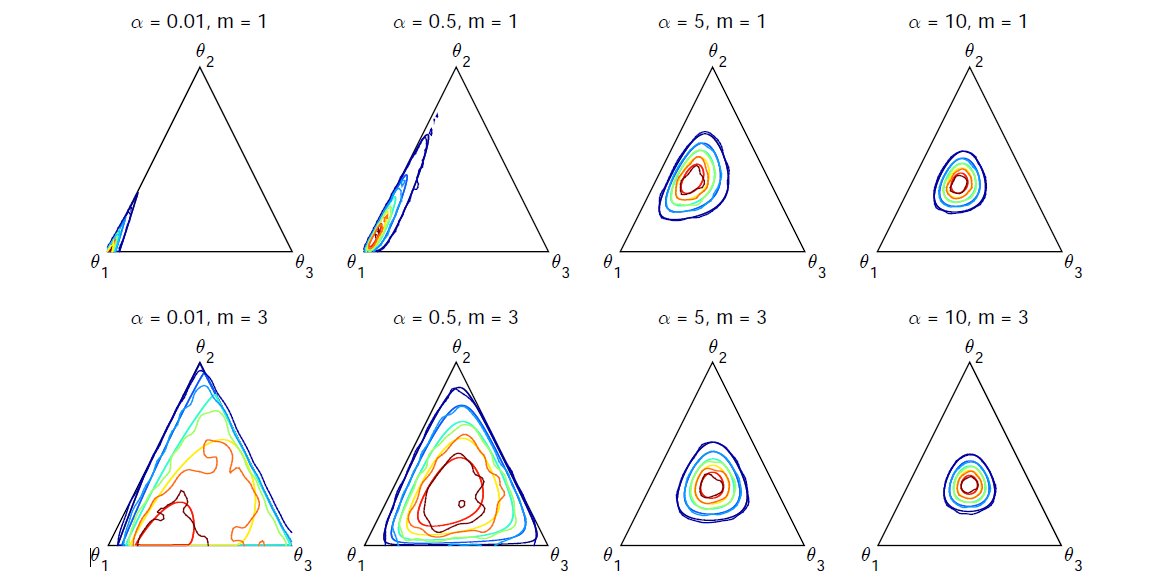
“… known to be asymptotically unbiased, bridge sampling technique produces biased estimates in practical usage for small to moderate sample sizes (…) the estimator yields positive bias that worsens with increasing distance between the two distributions. The second type of bias arises when the approximation density is determined from the posterior samples using the method of moments, resulting in a systematic underestimation of the normalizing constant.”

Recall that bridge sampling is based on a double trick with two samples x and y from two (unnormalised) densities f and g that are interverted in a ratio

of unbiased estimators of the inverse normalising constants. Hence biased. The more the less similar these two densities are. Special cases for ω include importance sampling [unbiased] and reciprocal importance sampling. Since the optimal version of the bridge weight ω is the inverse of the mixture of f and g, it makes me wonder at the performance of using both samples top and bottom, since as an aggregated sample, they also come from the mixture, as in Owen & Zhou (2000) multiple importance sampler. However, a quick try with a positive Normal versus an Exponential with rate 2 does not show an improvement in using both samples top and bottom (even when using the perfectly normalised versions)

morc=(sum(f(y)/(nx*dnorm(y)+ny*dexp(y,2)))+
            sum(f(x)/(nx*dnorm(x)+ny*dexp(x,2))))/(
  sum(g(x)/(nx*dnorm(x)+ny*dexp(x,2)))+
         sum(g(y)/(nx*dnorm(y)+ny*dexp(y,2))))

at least in terms of bias… Surprisingly (!) the bias almost vanishes for very different samples sizes either in favour of f or in favour of g. This may be a form of genuine defensive sampling, who knows?! At the very least, this ensures a finite variance for all weights. (The splitting approach introduced in the paper is a natural solution to create independence between the first sample and the second density. This reminded me of our two parallel chains in AMIS.)

commentaries in financial econometrics

My comment(arie)s on the moment approach to Bayesian inference by Ron Gallant have appeared, along with other comment(arie)s:

Invited Article
Reflections on the Probability Space Induced by Moment Conditions with
Implications for Bayesian Inference
A. Ronald Gallant . . . . . . . . . . . . . . . . . . . . . . . . . . . 229
Commentaries
Dante Amengual and Enrique Sentana .. . . . . . . . . . 248
John Geweke . . . . . . . . . . . . . . . . . . . . . . . . . . . . . . .253
Jae-Young Kim . . . . . . . . . . . . . . . . . . . . . . . . . . . . . . . . . . . . . . . . . . . . . . . . . 258
Oliver Linton and Ruochen Wu . . . . . . . . . . . . . . . . . . . . . . . . . . . . . . . . . . . . .261
Christian P. Robert . . . . . . . . . . . . . . . . . . . . . . . . . . . . . . . . . . . . . . . . . . . . . . 265
Christopher A. Sims . . . . . . . . . . . . . . . . . . . . . . . . . . . . . . . . . . . . . . . . . . . . . 272
Wei Wei and Asger Lunde . . . . . . . . . . . . . . . . . . . . . . . . . . . . . .  . . . . . . . . . .278
Author Response
A. Ronald Gallant . . . . . . . . . . . . . . . . . . . . . . . . . . . . . . . . . . . . . . . . . . . .284

While commenting on commentaries is formally bound to induce an infinite loop [or l∞p], I remain puzzled by the main point of the paper, which is that setting a structural distribution on a moment function Z(x,θ) plus a prior p(θ) induces a distribution on the pair (x,θ) in a possibly weaker σ-algebra. (The two distributions may actually be incompatible.) Handling this framework requires checking that a posterior exists, which sounds rather unnatural (even though we also have to check properness of the posterior). And the meaning of such a posterior remains unclear, as for instance in this assertion that (4) above is a likelihood, when it does not define a density in x but on the object inside the exponential.

“…it is typically difficult to determine whether there exists a p(x|θ) such that the implied distribution of m(x,θ) is the one stated, and if not, what damage is done thereby” J. Geweke (p.254)

estimating mixtures by polynomials

Sida Wang, Arun Tejasvi, and Chaganty Percy Liang have just arXived a paper about using the method of moments to estimate mixtures of distributions. Method that was introduced (?) by Pearson in 1894 for a Gaussian mixture and crab data. And studied in fair details by Bruce Lindsay and his co-authors, including his book, which makes it the more surprising that Bruce’s work is not mentioned at all in the paper. In particular the 1989 Annals of Statistics paper which connects the number of components with the rank of a moment matrix in exponential family and which made a strong impression on me at the time, just when I was starting to work on mixtures. The current paper addresses more specifically the combinatoric difficulty of solving the moment equation. The solution proceeds via a relaxed convex optimisation problem involving a moment matrix, the relaxation removing the rank condition that identifies the parameters of the mixture. While I am no expert in the resolution of the associated eigenvalue problem (Algorithm 1), I wonder at (i) the existence and convergence of a solution when using empirical moments. And (ii) the impact of the choice of the moment equations, on both existence and efficiency of the moment method. It is clearly not invariant by reparameterisation, hence parameterisation matters. It is even unclear to me how many terms should be used in the resolution: if a single dimension is acceptable, determining this dimension may prove a complex issue.

twilight zone [of statistics]

“I have decided that mixtures, like tequila, are inherently evil and should be avoided at all costs.” L. Wasserman

Larry Wasserman once remarked that finite mixtures were like the twilight zone of statistics, thanks to the numerous idiosyncrasies associated with such models. And George Casella had similar strong reservations about mixture estimation. Avi Feller and co-authors [including Natesh Pillai] have just arXived a paper on this topic, exhibiting shocking (!) properties of the MLE! Their core example is a mixture of two normal distributions with known common variance and known weight different from 0.5, which ensures identifiability. This is a favourite example of mine that we used for instance in our book Introducing Monte Carlo methods with R. If only because we can plot the likelihood and posterior surfaces. (Warning: I wrote those notes on an earlier version of the paper, so mileage may vary in terms of accuracy!)

The “shocking” discovery in the paper is that the MLE is wrong as often as not in selecting the sign of the difference Δ between both means, with an additional accumulation point at zero. The global mode may thus be in the wrong place for small enough sample sizes. And even for larger sizes: when the difference between the means is small the likelihood is likely to be unimodal with a mode quite close to zero. (An interesting remark is that the likelihood derivative is always zero at Δ=0 when considering the special case of both means equal to -Δ and to πΔ/(1-π), respectively, which implies that the overall mean of the mixture is equal to zero. A potential connection with our reparameterisation paper, maybe?)

The alternative proposed by Avi and his co-authors is to proceed through moments, i.e., to revert to Pearson (1892). There are however difficulties with this approach, first and foremost the non-uniqueness of the moment equations used to estimate Δ. For instance, the second cumulant equation chosen by the authors is not always defined as opposed to the third cumulant equation (why not using this third cumulant then). Which does not always produce the right sign… But, in a strange twist, the authors turn those deficiencies into signals for both pathologies (wrong sign and “pile-up” at zero).

“…the grid bootstrap yields an exact p-value for any valid test statistic.”

The most importance issue in this framework being in estimating the parameters, the authors opt for an approach based on tests, which is definitely surprising given the well-known deficiencies of standard tests in mixtures. The test chosen here is a Wald test with a statistic equal to the χ² version of the first cumulant differences. I am surprised that the χ² approximation works in such an unfriendly setting. And I do not understand how the grid is used, unless a certain degree of approximation is accepted, which takes us back to the “dark ages” of imposing a minimal distance Δ to achieve consistency, as in Ghosh and Sen (1985).

“..our concern about sign error is trivial in the Bayesian setting: the global mode is simply a poor summary of a multi-modal posterior. More broadly, the weak identification issues we highlight in this paper are not necessarily relevant to a strict Bayesian.”

A priori, I do not think pathologies of the MLE always transfer to Bayes estimators, unless one uses the MAP as an [poor] estimator. But using the MAP is not necessary since posterior means are meaningful in this identified setting, where label switching should not occur. However, running the same experiments with a Gaussian prior on both means and using the posterior mean as my estimator, I did obtain the same pathology of Bayes estimates [also produced in the supplementary material] not concentrating on the true value of the difference, but putting weight on the opposite value and at zero. Using a less standard prior inspired by David Rossell’s talk on non-local priors two weeks ago, which avoids a neighbourhood of zero, I did not get a much different picture as illustrated below:

Overall, I remain somewhat uncertain as to what to conclude from this pathological behaviour. When both means are close enough, the sign of the difference is often estimated wrongly. But that could simply mean that the means are not significantly different, for that sample size…

Moment conditions and Bayesian nonparametrics

Luke Bornn, Neil Shephard, and Reza Solgi (all from Harvard) have arXived a pretty interesting paper on simulating targets on a zero measure set. Although it is not initially presented this way, but rather in non-parametric terms as moment conditions

where θ is the parameter of the sampling distribution, constrained by the value of β. (Which also contains quantile regression.) The very problem of simulating under a hard constraint has been bugging me for years and it is hence very exciting to see them come up with a proposal towards solving this difficulty! Even though it is restricted here to observations with a finite support (hence allowing for the use of a parametric Dirichlet prior). One interesting extension (Section 3.6) processed in the paper is the case when the support is unknown, but finite, with some points in the support being unobserved. Maybe connecting with non-parametrics if a prior is added on the number of unobserved points.

The setting of constricting θ via a parameterised moment condition relates to moment defined econometrics models, in a similar spirit to Gallant’s paper I recently discussed, but equally to empirical likelihood, which would then benefit from a fully Bayesian treatment thanks to the approach advocated by the authors.

Despite the zero-measure difficulty, or more exactly the non-linear manifold structure of the parameter space, for instance

β = log {θ/(1-θ)}

the authors manage to define a “projected” [my words] measure on the set of admissible pairs (β,θ). In a sense this is related with the choice of a certain metric, but the so-called Hausdorff reference measure allows for an automated definition of the original prior. It took me a (wee) while to spot (p.7) that the starting point was not a (unconstrained) prior on that (unconstrained) pair (β,θ) but directly on the manifold

Which makes its construction a difficulty. Even though, as noted in Section 4, all that we need is a prior over θ since the Hausdorff-Jacobian identity defines the “joint”, in a sort of backward way. (This is a wee bit confusing in that β being a transform of θ, all we need is a prior over θ, but we nonetheless end up with a different density on the joint distribution on the pair (β,θ). Any connection with incompatible priors merged together into a consensus prior?) Another question extending the scope of the paper would be to define Jeffreys’ or reference priors in this manifold sense.

The authors also discuss (Section 4.3) the problem I originally thought they were processing, namely starting from an unconstrained pair (β,θ) and it corresponding prior. The projected prior can then be defined based on a version of the original density on the constrained space, but it is definitely arbitrary. In that sense the paper does not address the general problem.

“…traditional simulation algorithms will fail because the prior and the posterior of the model are supported on a zero Lebesgue measure set…” (p.10)

I somewhat resist this presentation through the measure zero set: once the prior is defined on a manifold, the fact that it is a measure zero set in a larger space is moot. Provided one can simulate a proposal over that manifold, e.g., a random walk, absolutely continuous wrt the same dominating measure, and compute or estimate a Metropolis-Hastings ratio of densities against a common measure, one can formally run MCMC on manifolds as well as regular Euclidean spaces. A first and theoretically straightforward (?) solution is to solve the constraint

in β=β(θ). Then the joint prior p(β,θ) can be projected by the Hausdorff projection into p(θ). For instance, in the case of the above logit transform, the projected density is

p(θ)=p(β,θ) {1+1/θ²(1-θ)²}½

In practice, the inversion may be too costly and Bornn et al. directly simulate the pair (β,θ) within the manifold capitalising on the fact that the constraint is linear in θ given β. Indeed, in this setting, β is unconstrained and θ can be simulated from a proposal restricted to the hyperplane. Gibbs-like.