a general framework for updating belief functions

Pier Giovanni Bissiri, Chris Holmes and Stephen Walker have recently arXived the paper related to Sephen’s talk in London for Bayes 250. When I heard the talk (of which some slides are included below), my interest was aroused by the facts that (a) the approach they investigated could start from a statistics, rather than from a full model, with obvious implications for ABC, & (b) the starting point could be the dual to the prior x likelihood pair, namely the loss function. I thus read the paper with this in mind. (And rather quickly, which may mean I skipped important aspects. For instance, I did not get into Section 4 to any depth. Disclaimer: I wasn’t nor is a referee for this paper!)

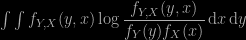
The core idea is to stick to a Bayesian (hardcore?) line when missing the full model, i.e. the likelihood of the data, but wishing to infer about a well-defined parameter like the median of the observations. This parameter is model-free in that some degree of prior information is available in the form of a prior distribution. (This is thus the dual of frequentist inference: instead of a likelihood w/o a prior, they have a prior w/o a likelihood!) The approach in the paper is to define a “posterior” by using a functional type of loss function that balances fidelity to prior and fidelity to data. The prior part (of the loss) ends up with a Kullback-Leibler loss, while the data part (of the loss) is an expected loss wrt to l(THETASoEUR,x), ending up with the definition of a “posterior” that is

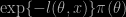
the loss thus playing the role of the log-likelihood.

I like very much the problematic developed in the paper, as I think it is connected with the real world and the complex modelling issues we face nowadays. I also like the insistence on coherence like the updating principle when switching former posterior for new prior (a point sorely missed in this book!) The distinction between M-closed M-open, and M-free scenarios is worth mentioning, if only as an entry to the Bayesian processing of pseudo-likelihood and proxy models. I am however not entirely convinced by the solution presented therein, in that it involves a rather large degree of arbitrariness. In other words, while I agree on using the loss function as a pivot for defining the pseudo-posterior, I am reluctant to put the same faith in the loss as in the log-likelihood (maybe a frequentist atavistic gene somewhere…) In particular, I think some of the choices are either hard or impossible to make and remain unprincipled (despite a call to the LP on page 7).  I also consider the M-open case as remaining unsolved as finding a convergent assessment about the pseudo-true parameter brings little information about the real parameter and the lack of fit of the superimposed model. Given my great expectations, I ended up being disappointed by the M-free case: there is no optimal choice for the substitute to the loss function that sounds very much like a pseudo-likelihood (or log thereof). (I thought the talk was more conclusive about this, I presumably missed a slide there!) Another great expectation was to read about the proper scaling of the loss function (since L and wL are difficult to separate, except for monetary losses). The authors propose a “correct” scaling based on balancing both faithfulness for a single observation, but this is not a completely tight argument (dependence on parametrisation and prior, notion of a single observation, &tc.)

The illustration section contains two examples, one of which is a full-size or at least challenging  genetic data analysis. The loss function is based on a logistic  pseudo-likelihood and it provides results where the Bayes factor is in agreement with a likelihood ratio test using Cox’ proportional hazard model. The issue about keeping the baseline function as unkown reminded me of the Robbins-Wasserman paradox Jamie discussed in Varanasi. The second example offers a nice feature of putting uncertainties onto box-plots, although I cannot trust very much the 95%  of the credibles sets. (And I do not understand why a unique loss would come to be associated with the median parameter, see p.25.)

Watch out: Tomorrow’s post contains a reply from the authors!

Initializing adaptive importance sampling with Markov chains

Another paper recently arXived by Beaujean and Caldwell elaborated on our population Monte Carlo papers (Cappé et al., 2005, Douc et al., 2007, Wraith et al., 2010) to design a more thorough starting distribution. Interestingly, the authors mention the fact that PMC is an EM-type algorithm to emphasize the importance of the starting distribution, as with “poor proposal, PMC fails as proposal updates lead to a consecutively poorer approximation of the target” (p.2). I had not thought of this possible feature of PMC, which indeed proceeds along integrated EM steps, and thus could converge to a local optimum (if not poorer than the start as the Kullback-Leibler divergence decreases).

The solution proposed in this paper is similar to the one we developed in our AMIS paper. An important part of the simulation is dedicated to the construction of the starting distribution, which is a mixture deduced from multiple Metropolis-Hastings runs. I find the method spends an unnecessary long time on refining this mixture by culling the number of components: down-the-shelf clustering techniques should be sufficient, esp. if one considers that the value of the target is available at every simulated point. This has been my pet (if idle) theory for a long while: we do not take (enough) advantage of this informative feature in our simulation methods… I also find the Student’s t versus Gaussian kernel debate (p.6) somehow superfluous: as we shown in Douc et al., 2007, we can process Student’s t distributions so we can as well work with those. And rather worry about the homogeneity assumption this choice implies: working with any elliptically symmetric kernel assumes a local Euclidean structure on the parameter space, for all components, and does not model properly highly curved spaces. Another pet theory of mine’s. As for picking the necessary number of simulations at each PMC iteration, I would add to the ESS and the survival rate of the components a measure of the Kullback-Leibler divergence, as it should decrease at each iteration (with an infinite number of particles).

Another interesting feature is in the comparison with Multinest, the current version of nested sampling, developed by Farhan Feroz. This is the second time I read a paper involving nested sampling in the past two days. While this PMC implementation does better than nested sampling on the examples processed in the paper, the Multinest outcome remains relevant, particularly because it handles multi-modality fairly well. The authors seem to think parallelisation is an issue with nested sampling, while I do see why: at the most naïve stage, several nested samplers can be run in parallel and the outcomes pulled together.

optimal direction Gibbs

An interesting paper appeared on arXiv today. Entitled On optimal direction gibbs sampling, by Andrés Christen, Colin Fox, Diego Andrés Pérez-Ruiz and Mario Santana-Cibrian, it defines optimality as picking the direction that brings the maximum independence between two successive realisations in the Gibbs sampler. More precisely, it aims at choosing the direction e that minimises the mutual information criterion

I have a bit of an issue about this choice because it clashes with measure theory. Indeed, in one Gibbs step associated with e the transition kernel is defined in terms of the Lebesgue measure over the line induced by e. Hence the joint density of the pair of successive realisations is defined in terms of the product of the Lebesgue measure on the overall space and of the Lebesgue measure over the line induced by e… While the product in the denominator is defined against the product of the Lebesgue measure on the overall space and itself. The two densities are therefore not comparable since not defined against equivalent measures… The difference between numerator and denominator is actually clearly expressed in the normal example (page 3) when the chain operates over a n dimensional space, but where the conditional distribution of the next realisation is one-dimensional, thus does not relate with the multivariate normal target on the denominator. I therefore do not agree with the derivation of the mutual information henceforth produced as (3).

The above difficulty is indirectly perceived by the authors, who note “we cannot simply choose the best direction: the resulting Gibbs sampler would not be irreducible” (page 5), an objection I had from an earlier page… They instead pick directions at random over the unit sphere and (for the normal case) suggest using a density over those directions such that

which cannot truly be called “optimal”.

More globally, searching for “optimal” directions (or more generally transforms) is quite a worthwhile idea, esp. when linked with adaptive strategies…

seminar at CREST on predictive estimation

On Thursday, March 08, Éric Marchand (from Université de Sherbrooke, Québec, where I first heard of MCMC!, and currently visiting Université de Montpellier 2) will give a seminar at CREST. It is scheduled at 2pm in ENSAE (ask the front desk for the room!) and is related to a recent EJS paper with Dominique Fourdrinier, Ali Righi, and Bill Strawderman: here is the abstract from the paper (sorry, the pictures from Roma are completely unrelated, but I could not resist!):

We consider the problem of predictive density estimation for normal models under Kullback-Leibler loss (KL loss) when the parameter space is constrained to a convex set. More particularly, we assume that

is observed and that we wish to estimate the density of

under KL loss when μ is restricted to the convex set C⊂ℝ^p. We show that the best unrestricted invariant predictive density estimator p̂_U is dominated by the Bayes estimator p̂_πC associated to the uniform prior π_C on C. We also study so called plug-in estimators, giving conditions under which domination of one estimator of the mean vector μ over another under the usual quadratic loss, translates into a domination result for certain corresponding plug-in density estimators under KL loss. Risk comparisons and domination results are also made for comparisons of plug-in estimators and Bayes predictive density estimators. Additionally, minimaxity and domination results are given for the cases where: (i) C is a cone, and (ii) C is a ball.

On optimality of kernels for ABC-SMC

This freshly arXived paper by Sarah Filippi, Chris Barnes, Julien Cornebise, and Michael Stumpf, is in the lineage of our 2009 Biometrika ABC-PMC (population Monte Carlo) paper with Marc Beaumont, Jean-Marie Cornuet and Jean-Michel Marin. (I actually missed the first posting while in Berlin last summer. Flying to Utah gave me the opportunity to read it at length!)  The  paper focusses on the impact of the transition kernel in our PMC scheme: while we used component-wise adaptive proposals, the paper studies multivariate adaptivity with a covariance matrix adapted from the whole population, or locally or from an approximation to the information matrix. The simulation study run in the paper shows that, even when accounting for the additional cost due to the derivation of the matrix, the multivariate adaptation can improve the acceptance rate by a fair amount. So this is an interesting and positive sequel to our paper (that I may well end up refereeing one of those days, like an earlier paper from some of the authors!)

The main criticism I may have about the paper is that the selection of the tolerance sequence is not done in an adaptive way, while it could, given the recent developments of Del Moral et al. and of Drovandri and Pettitt (as well as our even more recent still-un-arXived submission to Stat & Computing!). While the target is the same for all transition kernels, thus the comparison still makes sense as is, the final product is to build a complete adaptive scheme that comes as close as possible to the genuine posterior.

This paper also raised a new question: there is a slight distinction between the Kullback-Leibler divergence we used and the Kullback-Leibler divergence the authors use here. (In fact, we do not account for the change in the tolerance.) Now, since what only matters is the distribution of the current particles, and while the distribution on the past particles is needed to compute the double integral leading to the divergence, there is a complete freedom in the choice of this past distribution. As in Del Moral et al., the distribution L(θ:_t-1|θ_t) could therefore be chosen towards an optimal acceptance rate or something akin. I wonder if anyone ever looked at this…