Another harmonic mean

Yet another paper that addresses the approximation of the marginal likelihood by a truncated harmonic mean, a popular theme of mine. A 2020 paper by Johannes Reich, entitled Estimating marginal likelihoods from the posterior draws through a geometric identity and published in Monte Carlo Methods and Applications.

The geometric identity it aims at exploiting is that

for any (positive volume) compact set $A$. This is exactly the same identity as in an earlier and uncited 2017 paper by Ana Pajor, with the also quite similar (!) title Estimating the Marginal Likelihood Using the Arithmetic Mean Identity and which I discussed on the ‘Og, linked with another 2012 paper by Lenk. Also discussed here. This geometric or arithmetic identity is again related to the harmonic mean correction based on a HPD region A that Darren Wraith and myself proposed at MaxEnt 2009. And that Jean-Michel and I presented at Frontiers of statistical decision making and Bayesian analysis in 2010.

In this avatar, the set A is chosen close to an HPD region, once more, with a structure that allows for an exact computation of its volume. Namely an ellipsoid that contains roughly 50% of the simulations from the posterior (rather than our non-intersecting union of balls centered at the 50% HPD points), which assumes a Euclidean structure of the parameter space (or, in other words, depends on the parameterisation)In the mixture illustration, the author surprisingly omits Chib’s solution, despite symmetrised versions avoiding the label (un)switching issues. . What I do not get is how this solution gets around the label switching challenge in that set A remains an ellipsoid for multimodal posteriors, which means it either corresponds to a single mode [but then how can a simulation be restricted to a “single permutation of the indicator labels“?] or it covers all modes but also the unlikely valleys in-between.

 

meandering

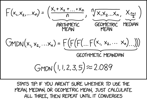
A bit of a misunderstanding from Randall Munroe and then some: the function F returns a triplet, hence G should return a triplet as well. Even if the limit does return three identical values. And he should have also included the (infamous) harmonic mean! And the subtext (behind the picture) mentions random forest statistics, using every mean one can think of and dropping those that are doing worse, while here all solutions return the same value, hence do not directly discriminate between the averages (and there is no objective function to create the nodes in the trees, &tc.).

Here is a test R code including the harmonic mean:

xkcd=function(x)c(mean(x),exp(mean(log(x))),median(x),1/mean(1/x))
xxxkcd=function(x,N=10)ifelse(rep(N==1,4),xkcd(x),xxxkcd(xkcd(x),N-1))
xxxkcd(rexp(11))
[1] 1.018197 1.018197 1.018197 1.018197

approximating evidence with missing data

Panayiota Touloupou (Warwick), Naif Alzahrani, Peter Neal, Simon Spencer (Warwick) and Trevelyan McKinley arXived a paper yesterday on Model comparison with missing data using MCMC and importance sampling, where they proposed an importance sampling strategy based on an early MCMC run to approximate the marginal likelihood a.k.a. the evidence. Another instance of estimating a constant. It is thus similar to our Frontier paper with Jean-Michel, as well as to the recent Pima Indian survey of James and Nicolas. The authors give the difficulty to calibrate reversible jump MCMC as the starting point to their research. The importance sampler they use is the natural choice of a Gaussian or t distribution centred at some estimate of θ and with covariance matrix associated with Fisher’s information. Or derived from the warmup MCMC run. The comparison between the different approximations to the evidence are done first over longitudinal epidemiological models. Involving 11 parameters in the example processed therein. The competitors to the 9 versions of importance samplers investigated in the paper are the raw harmonic mean [rather than our HPD truncated version], Chib’s, path sampling and RJMCMC [which does not make much sense when comparing two models]. But neither bridge sampling, nor nested sampling. Without any surprise (!) harmonic means do not converge to the right value, but more surprisingly Chib’s method happens to be less accurate than most importance solutions studied therein. It may be due to the fact that Chib’s approximation requires three MCMC runs and hence is quite costly. The fact that the mixture (or defensive) importance sampling [with 5% weight on the prior] did best begs for a comparison with bridge sampling, no? The difficulty with such study is obviously that the results only apply in the setting of the simulation, hence that e.g. another mixture importance sampler or Chib’s solution would behave differently in another model. In particular, it is hard to judge of the impact of the dimensions of the parameter and of the missing data.

rediscovering the harmonic mean estimator

When looking at unanswered questions on X validated, I came across a question where the author wanted to approximate a normalising constant

while simulating from the associated density, g. While seemingly unaware of the (huge) literature in the area, he re-derived [a version of] the harmonic mean estimate by considering the [inverted importance sampling] identity

when α is a probability density and by using for α the uniform over the whole range of the simulations from g. This choice of α obviously leads to an estimator with infinite variance when the support of g is unbounded, but the idea can be easily salvaged by using instead another uniform distribution, for instance on an highest density region, as we studied in our papers with Darren Wraith and Jean-Michel Marin. (Unfortunately, the originator of the question does not seem any longer interested in the problem.)

a remarkably simple and accurate method for computing the Bayes factor &tc.

This recent arXiv posting by Martin Weinberg and co-authors was pointed out to me by friends because of its title! It indeed sounded a bit inflated. And also reminded me of old style papers where the title was somehow the abstract. Like An Essay towards Solving a Problem in the Doctrine of Chances… So I had a look at it on my way to Gainesville. The paper starts from the earlier paper by Weinberg (2012) in Bayesian Analysis where he uses an HPD region to determine the Bayes factor by a safe harmonic mean estimator (an idea we already advocated earlier with Jean-Michel Marin in the San Antonio volume and with Darren Wraith in the MaxEnt volume). An extra idea is to try to optimise [against the variance of the resulting evidence] the region over which the integration is performed: “choose a domain that results in the most accurate integral with the smallest number of samples” (p.3). The authors proceed by volume peeling, using some quadrature formula for the posterior coverage of the region, either by Riemann or Lebesgue approximations (p.5). I was fairly lost at this stage and the third proposal based on adaptively managing hyperrectangles (p.7) went completely over my head! The sentence “the results are clearly worse with O(∞) errors, but are still remarkably better for high dimensionality”(p.11) did not make sense either… The method may thus be remarkably simple, but the paper is not written in a way that conveys this impression!