mostly MC [April]

Bayesian differential privacy for free?

“We are interested in the question of how we can build differentially-private algorithms within the Bayesian framework. More precisely, we examine when the choice of prior is sufficient to guarantee differential privacy for decisions that are derived from the posterior distribution (…) we show that the Bayesian statistician’s choice of prior distribution ensures a base level of data privacy through the posterior distribution; the statistician can safely respond to external queries using samples from the posterior.”

Recently I came across this 2016 JMLR paper of Christos Dimitrakakis et al. on “how Bayesian inference itself can be used directly to provide private access to data, with no modification.” Which comes as a surprise since it implies that Bayesian sampling would be enough, per se, to keep both the data private and the information it conveys available. The main assumption on which this result is based is one of Lipschitz continuity of the model density, namely that, for a specific (pseudo-)distance ρ

uniformly in θ over a set Θ with enough prior mass

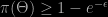
for an ε>0. In this case, the Kullback-Leibler divergence between the posteriors π(θ|x) and π(θ|y) is bounded by a constant times ρ(x,y). (The constant being 2L when Θ is the entire parameter space.) This condition ensures differential privacy on the posterior distribution (and even more on the associated MCMC sample). More precisely, (2L,0)-differentially private in the case Θ is the entire parameter space. While there is an efficiency issue linked with the result since the bound L being set by the model and hence immovable, this remains a fundamental result for the field (as shown by its high number of citations).

sequential neural likelihood estimation as ABC substitute

A JMLR paper by Papamakarios, Sterratt, and Murray (Edinburgh), first presented at the AISTATS 2019 meeting, on a new form of likelihood-free inference, away from non-zero tolerance and from the distance-based versions of ABC, following earlier papers by Iain Murray and co-authors in the same spirit. Which I got pointed to during the ABC workshop in Vancouver. At the time I had no idea as to autoregressive flows meant. We were supposed to hold a reading group in Paris-Dauphine on this paper last week, unfortunately cancelled as a coronaviral precaution… Here are some notes I had prepared for the meeting that did not take place.

“A simulator model is a computer program, which takes a vector of parameters θ, makes internal calls to a random number generator, and outputs a data vector x.”

Just the usual generative model then.

“A conditional neural density estimator is a parametric model q(.|φ) (such as a neural network) controlled by a set of parameters φ, which takes a pair of datapoints (u,v) and outputs a conditional probability density q(u|v,φ).”

Less usual, in that the outcome is guaranteed to be a probability density.

“For its neural density estimator, SNPE uses a Mixture Density Network, which is a feed-forward neural network that takes x as input and outputs the parameters of a Gaussian mixture over θ.”

In which theoretical sense would it improve upon classical or Bayesian density estimators? Where are the error evaluation, the optimal rates, the sensitivity to the dimension of the data? of the parameter?

“Our new method, Sequential Neural Likelihood (SNL), avoids the bias introduced by the proposal, by opting to learn a model of the likelihood instead of the posterior.”

I do not get the argument in that the final outcome (of using the approximation within an MCMC scheme) remains biased since the likelihood is not the exact likelihood. Where is the error evaluation? Note that in the associated Algorithm 1, the learning set is enlarged on each round, as in AMIS, rather than set back to the empty set ∅ on each round.

“…given enough simulations, a sufficiently flexible conditional neural density estimator will eventually approximate the likelihood in the support of the proposal, regardless of the shape of the proposal. In other words, as long as we do not exclude parts of the parameter space, the way we propose parameters does not bias learning the likelihood asymptotically. Unlike when learning the posterior, no adjustment is necessary to account for our proposing strategy.”

This is a rather vague statement, with the only support being that the Monte Carlo approximation to the Kullback-Leibler divergence does converge to its actual value, i.e. a direct application of the Law of Large Numbers! But an interesting point I informally made a (long) while ago that all that matters is the estimate of the density at x⁰. Or at the value of the statistic at x⁰. The masked auto-encoder density estimator is based on a sequence of bijections with a lower-triangular Jacobian matrix, meaning the conditional density estimate is available in closed form. Which makes it sounds like a form of neurotic variational Bayes solution.

The paper also links with ABC (too costly?), other parametric approximations to the posterior (like Gaussian copulas and variational likelihood-free inference), synthetic likelihood, Gaussian processes, noise contrastive estimation… With experiments involving some of the above. But the experiments involve rather smooth models with relatively few parameters.

“A general question is whether it is preferable to learn the posterior or the likelihood (…) Learning the likelihood can often be easier than learning the posterior, and it does not depend on the choice of proposal, which makes learning easier and more robust (…) On the other hand, methods such as SNPE return a parametric model of the posterior directly, whereas a further inference step (e.g. variational inference or MCMC) is needed on top of SNL to obtain a posterior estimate”

A fair point in the conclusion. Which also mentions the curse of dimensionality (both for parameters and observations) and the possibility to work directly with summaries.

Getting back to the earlier and connected Masked autoregressive flow for density estimation paper, by Papamakarios, Pavlakou and Murray:

“Viewing an autoregressive model as a normalizing flow opens the possibility of increasing its flexibility by stacking multiple models of the same type, by having each model provide the source of randomness for the next model in the stack. The resulting stack of models is a normalizing flow that is more flexible than the original model, and that remains tractable.”

Which makes it sound like a sort of a neural network in the density space. Optimised by Kullback-Leibler minimisation to get asymptotically close to the likelihood. But a form of Bayesian indirect inference in the end, namely an MLE on a pseudo-model, using the estimated model as a proxy in Bayesian inference…

Expectation Propagation as a Way of Life on-line

After a rather extended shelf-life, our paper expectation propagation as a way of life: a framework for Bayesian inference on partitioned data which was started when Andrew visited Paris in… 2014!, and to which I only marginally contributed, has now appeared in JMLR! Which happens to be my very first paper in this journal.

7 years later…