mean simulations

A rather intriguing question on X validated, namely a simulation approach to sampling a bivariate distribution fully specified by one conditional p(x|y) and the symmetric conditional expectation IE[Y|X=x]. The book Conditional Specification of Statistical Models, by Arnold, Castillo and Sarabia, as referenced by and in the question, contains (§7.7) illustrations of such cases. As for instance with some power series distribution on ℕ but also for some exponential families (think Laplace transform). An example is when

which means X conditional on Y=y is exponential E(λy). The expectation IE[Y|X=x] is then sufficient to identify the joint. As I figured out before checking the book, this result is rather immediate to establish by solving a linear system, but it does not help in finding a way to simulating the joint. (I am afraid it cannot be connected to the method of simulated moments!)

 

partial rankings and aggregate ranks

When interviewing impressive applicants from a stunning variety of places and background for fellows in our Data Science for Social Good program (in Warwick and Kaiserslautern) this summer, we came through the common conundrum of comparing ranks while each of us only meeting a subset of the candidates. Over a free morning, I briefly thought of the problem (while swimming) and then wrote a short R code to infer about an aggregate ranking, ρ, based on a simple model, namely a Poisson distribution on the distance between an individual’s ranking and the aggregate

a uniform distribution on the missing ranks as well as on the aggregate, and a non-informative prior on λ. Leading to a three step Gibbs sampler for the completion and the simulation of ρ and λ.

I am aware that the problem has been tackled in many different ways, including Bayesian ones (as in Deng et al., 2014) and local ones, but this was a fun exercise. Albeit we did not use any model in the end!

simplified Bayesian analysis

A colleague from Dauphine sent me a paper by Carlo Graziani on a Bayesian analysis of vaccine efficiency, asking for my opinion. The Bayesian side is quite simple: given two Poisson observations, N~P(μ) and M~P(ν), there exists a reparameterisation of (μ,ν) into

e=1-μ/rν  and  λ=ν(1+(1-e)r)=μ+ν

vaccine efficiency and expectation of N+M, respectively, when r is the vaccine-to-placebo ratio of person-times at risk, ie the ratio of the numbers of participants in each group. Reparameterisation such that the likelihood factorises into a function of e and a function of λ. Using a product prior for this parameterisation leads to a posterior on e times a posterior on λ. This is a nice remark, which may have been made earlier (as for instance another approach to infer about e while treating λ as a nuisance parameter is to condition on N+M). The paper then proposes as an application of this remark an analysis of the results of three SARS-Cov-2 vaccines, meaning using the pairs (N,M) for each vaccine and deriving credible intervals, which sounds more like an exercise in basic Bayesian inference than a fundamental step in assessing the efficiency of the vaccines…

Buffon machines

By chance I came across a 2010 paper entitled On Buffon Machines and Numbers by Philippe Flajolet, Maryse Pelletier and Michèle Soria. Which relates to Bernoulli factories, a related riddle, and the recent paper by Luis Mendo I reviewed here. What the authors call a Buffon machine is a device that produces a perfect simulation of a discrete random variable out of a uniform bit generator. Just like (George Louis Leclerc, comte de) Buffon’s needle produces a Bernoulli outcome with success probability π/4. out of a real Uniform over (0,1). Turned into a sequence of Uniform random bits.

“Machines that always halt can only produce Bernoulli distributions whose parameter is a dyadic rational.”

When I first read this sentence it seemed to clash with the earlier riddle, until I realised the later started from a B(p) coin to produce a fair coin, while this paper starts with a fair coin.

The paper hence aims at a version of the Bernoulli factory problem (see Definition 2), although the term is only mentioned at the very end, with the added requirement of simplicity and conciseness translated as a finite expected number of draws and possibly an exponential tail.

It first recalls the (Forsythe–)von Neumann method of generating exponential (and other) variates out of a Uniform generator (see Section IV.2 in Devroye’s generation bible). Expanded into a general algorithm for generating discrete random variables whose pmf’s are related to permutation cardinals,

if the Bernoulli generator has probability λ. These include the Poisson and the logarithmic distributions and as a side product Bernoulli distributions with some logarithmic, exponential and trigonometric transforms of λ.

As a side remark, a Bernoulli generator with probability 1/π is derived from Ramanujan identity

as “a discrete analogue of Buffon’s original. In a neat connection with Mendo’s paper, the authors of this 2010 paper note that Euler’s constant does not appear to be achievable by a Buffon machine.

Probability and Bayesian modeling [book review]

Probability and Bayesian modeling is a textbook by Jim Albert [whose reply is included at the end of this entry] and Jingchen Hu that CRC Press sent me for review in CHANCE. (The book is also freely available in bookdown format.) The level of the textbook is definitely most introductory as it dedicates its first half on probability concepts (with no measure theory involved), meaning mostly focusing on counting and finite sample space models. The second half moves to Bayesian inference(s) with a strong reliance on JAGS for the processing of more realistic models. And R vignettes for the simplest cases (where I discovered R commands I ignored, like dplyr::mutate()!).

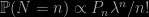
As a preliminary warning about my biases, I am always reserved at mixing introductions to probability theory and to (Bayesian) statistics in the same book, as I feel they should be separated to avoid confusion. As for instance between histograms and densities, or between (theoretical) expectation and (empirical) mean. I therefore fail to relate to the pace and tone adopted in the book which, in my opinion, seems to dally on overly simple examples [far too often concerned with food or baseball] while skipping over the concepts and background theory. For instance, introducing the concept of subjective probability as early as page 6 is laudable but I doubt it will engage fresh readers when describing it as a measurement of one’s “belief about the truth of an event”, then stressing that “make any kind of measurement, one needs a tool like a scale or ruler”. Overall, I have no particularly focused criticisms on the probability part except for the discrete vs continuous imbalance. (With the Poisson distribution not covered in the Discrete Distributions chapter. And the “bell curve” making a weird and unrigorous appearance there.) Galton’s board (no mention found of quincunx) could have been better exploited towards the physical definition of a prior, following Steve Stiegler’s analysis, by adding a second level. Or turned into an R coding exercise. In the continuous distributions chapter, I would have seen the cdf coming first to the pdf, rather than the opposite. And disliked the notion that a Normal distribution was supported by an histogram of (marathon) running times, i.e. values lower bounded by 122 (at the moment). Or later (in Chapter 8) for Roger Federer’s serving times. Incidentally, a fun typo on p.191, at least fun for LaTeX users, as

with an extra space between `\’ and `mid’! (I also noticed several occurrences of the unvoidable “the the” typo in the last chapters.) The simulation from a bivariate Normal distribution hidden behind a customised R function sim_binom() when it could have been easily described as a two-stage hierarchy. And no comment on the fact that a sample from Y-1.5X could be directly derived from the joint sample. (Too unconscious a statistician?)

When moving to Bayesian inference, a large section is spent on very simple models like estimating a proportion or a mean, covering both discrete and continuous priors. And strongly focusing on conjugate priors despite giving warnings that they do not necessarily reflect prior information or prior belief. With some debatable recommendation for “large” prior variances as weakly informative or (worse) for Exp(1) as a reference prior for sample precision in the linear model (p.415). But also covering Bayesian model checking either via prior predictive (hence Bayes factors) or posterior predictive (with no mention of using the data twice). A very marginalia in introducing a sufficient statistic for the Normal model. In the Normal model checking section, an estimate of the posterior density of the mean is used without (apparent) explanation.

“It is interesting to note the strong negative correlation in these parameters. If one assigned informative independent priors on ${\beta }_{\mathrm{⁰}}$and ${\beta }_{\mathrm{¹}}$, these prior beliefs would be counter to the correlation between the two parameters observed in the data.”

For the same reasons of having to cut on mathematical validation and rigour, Chapter 9 on MCMC is not explaining why MCMC algorithms are converging outside of the finite state space case. The proposal in the algorithmic representation is chosen as a Uniform one, since larger dimension problems are handled by either Gibbs or JAGS. The recommendations about running MCMC do not include how many iterations one “should” run (or other common queries on Stack eXchange), albeit they do include the sensible running multiple chains and comparing simulated predictive samples with the actual data as a  model check. However, the MCMC chapter very quickly and inevitably turns into commented JAGS code. Which I presume would require more from the students than just reading the available code. Like JAGS manual. Chapter 10 is mostly a series of examples of Bayesian hierarchical modeling, with illustrations of the shrinkage effect like the one on the book cover. Chapter 11 covers simple linear regression with some mentions of weakly informative priors,  although in a BUGS spirit of using large [enough?!] variances: “If one has little information about the location of a regression parameter, then the choice of the prior guess ${\mu }^{}$ is not that important and one chooses a large value for the prior standard deviation $s^{}$. So the regression intercept and slope are each assigned a Normal prior with a mean of 0 and standard deviation equal to the large value of 100.” (p.415). Regardless of the scale of y? Standardisation is covered later in the chapter (with the use of the R function scale()) as part of constructing more informative priors, although this sounds more like data-dependent priors to me in the sense that the scale and location are summarily estimated by empirical means from the data. The above quote also strikes me as potentially confusing to the students, as it does not spell at all how to design a joint distribution on the linear regression coefficients that translate the concentration of these coefficients along y̅=β⁰+β¹x̄. Chapter 12 expands the setting to multiple regression and generalised linear models, mostly consisting of examples. It however suggests using cross-validation for model checking and then advocates DIC (deviance information criterion) as “to approximate a model’s out-of-sample predictive performance” (p.463). If only because it is covered in JAGS, the definition of the criterion being relegated to the last page of the book. Chapter 13 concludes with two case studies, the (often used) Federalist Papers analysis and a baseball career hierarchical model. Which may sound far-reaching considering the modest prerequisites the book started with.

In conclusion of this rambling [lazy Sunday] review, this is not a textbook I would have the opportunity to use in Paris-Dauphine but I can easily conceive its adoption for students with limited maths exposure. As such it offers a decent entry to the use of Bayesian modelling, supported by a specific software (JAGS), and rightly stresses the call to model checking and comparison with pseudo-observations. Provided the course is reinforced with a fair amount of computer labs and projects, the book can indeed achieve to properly introduce students to Bayesian thinking. Hopefully leading them to seek more advanced courses on the topic.

Update: Jim Albert sent me the following precisions after this review got on-line:

Thanks for your review of our recent book.  We had a particular audience in mind, specifically undergraduate American students with some calculus background who are taking their first course in probability and statistics.  The traditional approach (which I took many years ago) teaches some probability one semester and then traditional inference (focusing on unbiasedness, sampling distributions, tests and confidence intervals) in the second semester.  There didn’t appear to be any Bayesian books at that calculus-based undergraduate level and that motivated the writing of this book.  Anyway, I think your comments were certainly fair and we’ve already made some additions to our errata list based on your comments.

[Disclaimer about potential self-plagiarism: this post or an edited version will eventually appear in my Books Review section in CHANCE. As appropriate for a book about Chance!]